OpenROAD Flow Scripts Tutorial#

Introduction#

This document describes a tutorial to run the complete OpenROAD flow from RTL-to-GDS using OpenROAD Flow Scripts. It includes examples of useful design and manual usage in key flow stages to help users gain a good understanding of the OpenROAD application flow, data organization, GUI and commands.

This is intended for:

Beginners or new users with some understanding of basic VLSI design flow. Users will learn the basics of installation to use OpenROAD-flow-scripts for the complete RTL-to-GDS flow from here.
Users already familiar with the OpenROAD application and flow but would like to learn more about specific features and commands.

User Guidelines#

This tutorial requires a specific directory structure built by OpenROAD-flow-scripts (ORFS). Do not modify this structure or underlying files since this will cause problems in the flow execution.
User can run the full RTL-to-GDS flow and learn specific flow sections independently. This allows users to learn the flow and tool capabilities at their own pace, time and preference.
Results shown, such as images or outputs of reports and logs, could vary based on release updates. However, the main flow and command structure should generally apply.

Note: Please submit any problem found under Issues in the GitHub repository here.

Getting Started#

This section describes the environment setup to build OpenROAD-flow-scripts and get ready to execute the RTL-to-GDS flow of the open-source design ibex using the sky130hd technology.

ibex is a 32 bit RISC-V CPU core (RV32IMC/EMC) with a two-stage pipeline.

Setting Up The Environment#

Use the bash shell to run commands and scripts.

OpenROAD-flow-scripts Installation#

To install OpenROAD-flow-scripts, refer to the Build or installing ORFS Dependencies documentation.

In general, we recommend using Docker for an efficient user experience. Install OpenROAD-flow-scripts using a docker as described here Build from sources using Docker.

Note

If you need to update an existing OpenROAD-flow-scripts installation, follow instructions from here.

OpenROAD-flow-scripts installation is complete.

Running OpenROAD-flow-scripts inside the Docker#

Launch the docker with OpenROAD-flow-scripts container as follows:

docker run --rm -it -u $(id -u ${USER}):$(id -g ${USER}) -v $(pwd)/flow:/OpenROAD-flow-scripts/flow openroad/flow-ubuntu22-builder

Verifying the Docker based Installation#

To verify the installation run the built-in example design as follows:

cd flow
make

A successful run end with the log:

[INFO] Writing out GDS/OAS 'results/nangate45/gcd/base/6_1_merged.gds'
Elapsed time: 0:10.44[h:]min:sec. CPU time: user 2.17 sys 0.54 (26%). Peak memory: 274184KB.
cp results/nangate45/gcd/base/6_1_merged.gds results/nangate45/gcd/base/6_final.gds
Log                       Elapsed seconds
1_1_yosys                          2
3_3_place_gp                       1
4_1_cts                            8
5_2_route                   10
6_1_merge                         10
6_report                           3

Configuring The Design#

This section shows how to set up the necessary platform and design configuration files to run the complete RTL-to-GDS flow using OpenROAD-flow-scripts for ibex design.

cd flow

Platform Configuration#

View the platform configuration file setup for default variables for sky130hd.

less ./platforms/sky130hd/config.mk

The config.mk file has all the required variables for the sky130 platform and hence it is not recommended to change any variable definition here. You can view the sky130hd platform configuration here.

Refer to the Flow variables document for details on how to use platform and design specific environment variables in OpenROAD-flow-scripts to customize and configure your design flow.

Design Configuration#

View the default design configuration of ibex design:

less ./designs/sky130hd/ibex/config.mk

You can view ibex design config.mk here.

Note

The following design-specific configuration variables are required to specify main design inputs such as platform, top-level design name and constraints. We will use default configuration variables for this tutorial.

Variable Name	Description
`PLATFORM`	Specifies Process design kit.
`DESIGN_NAME`	The name of the top-level module of the design
`VERILOG_FILES`	The path to the design Verilog files
`SDC_FILE`	The path to design `.sdc` file
`CORE_UTILIZATION`	The core utilization percentage.
`PLACE_DENSITY`	The desired placement density of cells. It reflects how spread the cells would be on the core area. 1 = closely dense. 0 = widely spread

Note

To add a new design to the flow, refer to the document here. This step is for advanced users. If you are a beginner, first understand the flow by completing this tutorial and come back to this step later to add a new design.

Timing Constraints#

View timing constraints specified in the .sdc file here.

less ./designs/sky130hd/ibex/constraint.sdc

For ibex design, we simply use the clock definition as follows as a minimum required timing constraint.

create_clock -name core_clock -period 17.4 [get_ports {clk_i}]

Design Input Verilog#

The Verilog input files are located in ./designs/src/ibex/

The design is defined in ibex_core.v available here.

Refer to the ibex design README.md here.

Running The Automated RTL-to-GDS Flow#

This section describes the complete execution of the design flow from RTL-to-GDS. The OpenROAD application executes the entire autonomous flow using Tcl scripts that invoke open-sourced tools, from synthesis to the final .gds file creation, without requiring human intervention. However, in this tutorial, the user will learn both the automated and a few interactive ways to run Tcl commands for important flow stages.

From the OpenROAD-flow-scripts directory, users can access individual flow stages, respective tools and the corresponding README.md for tool commands, configuration examples using the Tcl interface and other such details.

Design Goals#

Run the ibex design in OpenROAD-flow-scripts automated flow from RTL-to-GDS using sky130hd. Find ibex design details here and the design goals are:

Area

Minimum Required Die size: 0 0 798 800 (in micron)
Core size: 2 2 796 798 (in micron)

Timing

Clock period to meet timing: 17.4 (in ns)

ibex takes approximately 8 minutes on a machine with 8-cores and 16GB RAM. The runtime will vary based on your configuration.

Change your current directory to the flow directory.

cd flow

Run the complete flow with:

make DESIGN_CONFIG=./designs/sky130hd/ibex/config.mk

As the flow executes, check out the OpenROAD-flow-scripts directory contents and their significance.

OpenROAD-flow-scripts can generally restart from a previous partial run. If you have errors which prevent restarting the flow, you may try deleting all generated files and start a fresh run. Errors can occur if a tool crashes or is killed while writing a file. The files for sky130hd/ibex as an example can be deleted with:

make clean_all DESIGN_CONFIG=./designs/sky130hd/ibex/config.mk

You can also delete files related to individual stages of RTL to GDSII conversion like synthesis, floorplanning, macro placement, clock tree synthesis, routing and layout generation with clean_synth, clean_floorplan, clean_place, clean_cts, clean_route, and clean_finish, respectively.

Viewing OpenROAD-flow-scripts Directory Structure And Results#

Open a new tab in the terminal and explore the directory structure in flow by typing ls command to view its contents:

designs logs Makefile objects platforms reports results scripts test util

Navigate through each of the sub-directories above to understand how underlying files are organized.

designs/sky130hd/ibex Files include: designs make file and SDC file for the sky130hd platform and other files for autotuner and metrics.

autotuner.json config.mk constraint_doe.sdc constraint.sdc metadata-base-ok.json rules.json

platforms Includes public PDKs supported by OpenROAD flow

asap7 nangate45 sky130hd sky130hs sky130io sky130ram

objects/sky130hd/ibex/base Includes ABC constraints and all the temporary library files used for the completion flow

abc.constr klayout.lyt klayout_tech.lef lib

logs/sky130hd/ibex/base Logs directory, which contains log files for each flow stage.

`logs`
`1_1_yosys.log`	`3_1_place_gp.log`	`5_2_route.log`
`2_1_floorplan.log`	`3_2_place_iop.log`	`6_1_merge.log`
`2_2_floorplan_io.log`	`3_3_resizer.log`	`6_report.log`
`2_3_tdms_place.log`	`3_4_opendp.log`
`2_4_floorplan_macro.log`	`4_1_cts.log`
`2_5_floorplan_tapcell.log`	`4_2_cts_fillcell.log`
`2_6_floorplan_pdn.log`	`5_1_grt.log`

results/sky130hd/ibex/base Results directory which contains .v/.sdc/.odb/.def/.spef files

`results`
`1_1_yosys.v`	`3_1_place_gp.odb`	`5_route.sdc`
`1_synth.sdc`	`3_2_place_iop.odb`	`6_1_fill.odb`
`1_synth.v`	`3_3_place_resized.odb`	`6_1_fill.sdc`
`2_1_floorplan.odb`	`3_4_place_dp.odb`	`6_1_merged.gds`
`2_2_floorplan_io.odb`	`3_place.odb`	`6_final.odb`
`2_3_floorplan_tdms.odb`	`3_place.sdc`	`6_final.gds`
`2_4_floorplan_macro.odb`	`4_1_cts.odb`	`6_final.sdc`
`2_5_floorplan_tapcell.odb`	`4_2_cts_fillcell.odb`	`6_final.spef`
`2_6_floorplan_pdn.odb`	`4_cts.odb`	`6_final.v`
`2_floorplan.odb`	`4_cts.sdc`	`output_guide.mod`
`2_floorplan.sdc`	`4_cts.v`	`route.guide`
`2_floorplan.v`	`5_route.odb`	`updated_clks.sdc`

reports/sky130hd/ibex/base Reports directory, which contains congestion report, DRC report, design statistics and antenna log for reference.

`reports`
`congestion.rpt`	`VDD.rpt`	`VSS.rpt`
`5_route_drc.rpt`	`final_clocks.webp`	`final_placement.webp`
`antenna.log`	`final_clocks.webp`	`final.webp`
`synth_stat.txt`	`synth_check.txt`	`final_resizer.webp`

The table below briefly describes the reports directory files.

File Name	Description
`congestion.rpt`	Gloabl routing congestion if occurred.
`5_route_drc.rpt`	DRC violations if occurred.
`final_clocks.webp`	OR extracted image reference after clock tree synthesis.
`final_resizer.webp`	OR extracted image reference after resizer.
`synth_check.txt`	Synthesis warning/error messages.
`antenna.log`	Antenna check log report.
`final_placement.webp`	Extracted image after final placement.
`final.webp`	Extracted image after routing.
`synth_stat.txt`	Post synthesis design statistics log saved here.

The flow completes with the message below by creating a merged final GDS file.

[INFO] Writing out GDS/OAS
'results/sky130hd/ibex/base/6_1_merged.gds'
cp results/sky130hd/ibex/base/6_1_merged.gds
results/sky130hd/ibex/base/6_final.gds

Viewing Results And Logs#

OpenROAD-flow-scripts prepends a prefix to each flow stage, as shown below, to indicate the position in the RTL-GDS flow. This makes it easier to understand and debug each flow stage in case of failure.

View ibex design logs:

ls logs/sky130hd/ibex/base/

The log structure is as follows:

`logs`
`1_1_yosys.log`	`3_1_place_gp.log`	`5_2_route.log`
`2_1_floorplan.log`	`3_2_place_iop.log`	`6_1_merge.log`
`2_2_floorplan_io.log`	`3_3_resizer.log`	`6_report.log`
`2_3_tdms_place.log`	`3_4_opendp.log`
`2_4_floorplan_macro.log`	`4_1_cts.log`
`2_5_floorplan_tapcell.log`	`4_2_cts_fillcell.log`
`2_6_floorplan_pdn.log`	`5_1_grt.log`

Area#

View design area and its core utilization:

make gui_final
report_design_area

View the resulting area as:

Design area 191262 u^2 30% utilization.

Timing#

Users can view flow results using the command interface from the shell or the OpenROAD GUI to visualize further and debug. Learn more about the GUI.

make gui_final

Use the following commands in the Tcl Commands section of GUI:

report_worst_slack
report_tns
report_wns

Note the worst slack, total negative slack and worst negative slack:

worst slack -0.99
tns -1.29
wns -0.99

Learn more about visualizing and tracing time paths across the design hierarchy refer to the OpenROAD GUI.

Power#

Use the report command to view individual power components i.e. sequential, combinational, macro and power consumed by I/O pads.

report_power

The power output is as follows:

--------------------------------------------------------------------------
Group                  Internal  Switching    Leakage      Total
                          Power      Power      Power      Power
----------------------------------------------------------------
Sequential             5.58e-03   6.12e-04   1.67e-08   6.19e-03  19.0%
Combinational          9.23e-03   1.71e-02   4.90e-08   2.63e-02  81.0%
Macro                  0.00e+00   0.00e+00   0.00e+00   0.00e+00   0.0%
Pad                    0.00e+00   0.00e+00   0.00e+00   0.00e+00   0.0%
----------------------------------------------------------------
Total                  1.48e-02   1.77e-02   6.57e-08   3.25e-02 100.0%
                          45.6%      54.4%       0.0%

OpenROAD GUI#

The GUI allows users to select, control, highlight and navigate the design hierarchy and design objects (nets, pins, instances, paths, etc.) through detailed visualization and customization options. Find details on how to use the GUI. All the windows aside from the layout are docking windows that can be undocked. Also it can be closed and reopened from the Windows menu.

Note: When you are using remote access, you will need to include -Y (or -X) option in your command to enable X11 applications to function properly over the network. By using the command “ssh -Y” followed by the remote servers’ address or hostname, you can establish a secure connection and activate X11 forwarding. This feature enables you to run graphical programs on the remote server and have their windows display on your local machines desktop environment.

In this section, learn how to:

Visualize design hierarchy
Load ODB files for floorplan and layout visualization
Trace the synthesized clock tree to view hierarchy and buffers
Use heat maps to view congestion and observe the effect of placement
View and trace critical timing paths
Set display control options
Zoom to object from inspector

If you have completed the RTL-GDS flow, then proceed to view the final GDS file under results directory ./results/sky130hd/ibex/base/

For the ibex design uncomment the DESIGN_CONFIG variable in the Makefile available here.

# DESIGN_CONFIG=./designs/sky130hd/gcd/config.mk
DESIGN_CONFIG=./designs/sky130hd/ibex/config.mk
# DESIGN_CONFIG=./designs/sky130hd/aes/config.mk

make gui_final

Viewing Layout Results#

The make gui_final command target successively reads and loads the technology .odb files and the parasitics and invokes the GUI in these steps:

Reads and loads .odb files.
Loads .spef (parasitics).

The figure below shows the post-routed DEF for the ibex design.

ibex_final_db

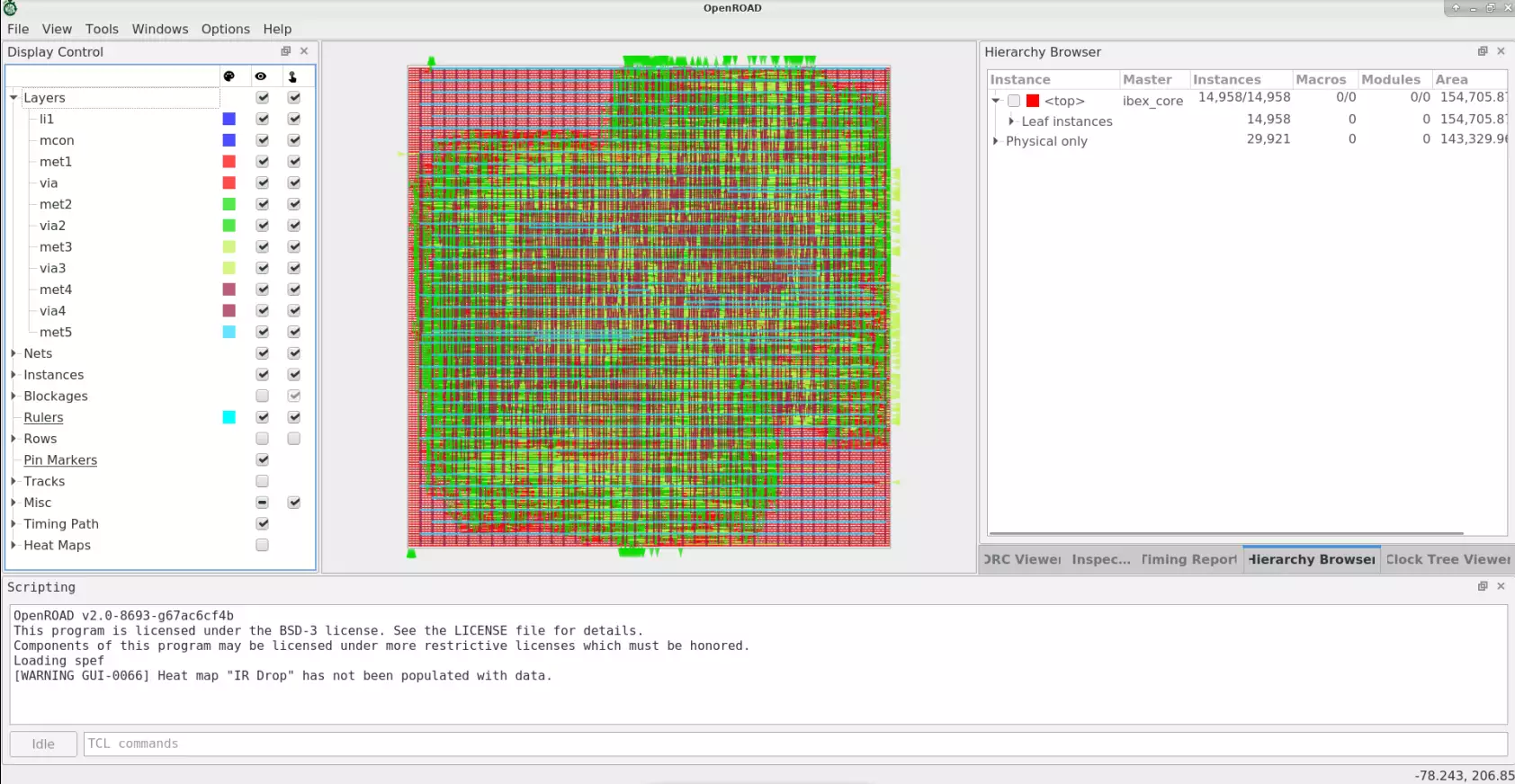
Visualizing Design Objects And Connectivity#

Note the Display Control window on the LHS that shows buttons for color, visibility and selection options for various design objects: Layers, Nets, Instances, Blockages, Heatmaps, etc.

The Inspector window on the RHS allows users to inspect details of selected design objects and the timing report.

Try selectively displaying (show/hide) various design objects through the display control window and observing their impact on the display.

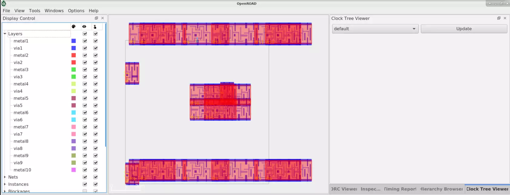
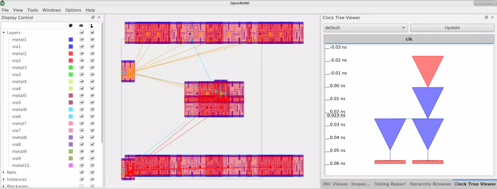
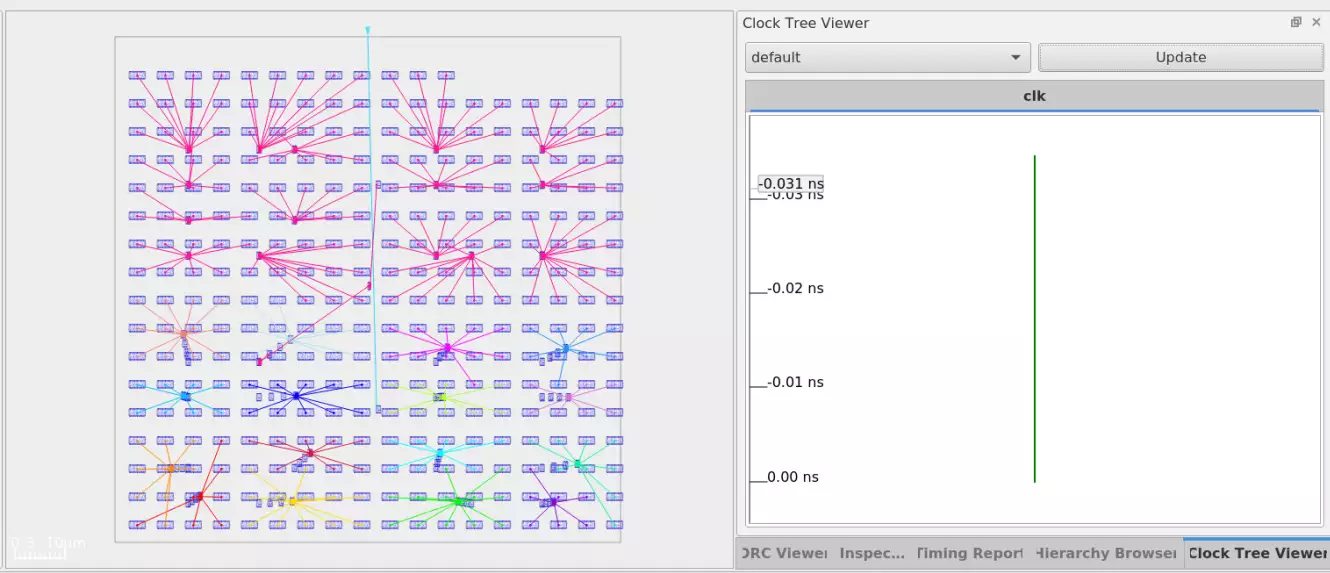
Tracing The Clock Tree#

View the synthesized clock tree for ibex design:

From the top Toolbar Click Windows -> Clock Tree Viewer

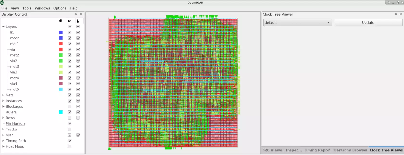
On RHS, click Clock Tree Viewer and top right corner, click Update to view the synthesized clock tree of your design.

View clock tree structure below, the user needs to disable the metal Layers section on LHS as shown below.

From the top Toolbar, click on the Windows menu to select/hide different view options of Scripting, Display control, etc.

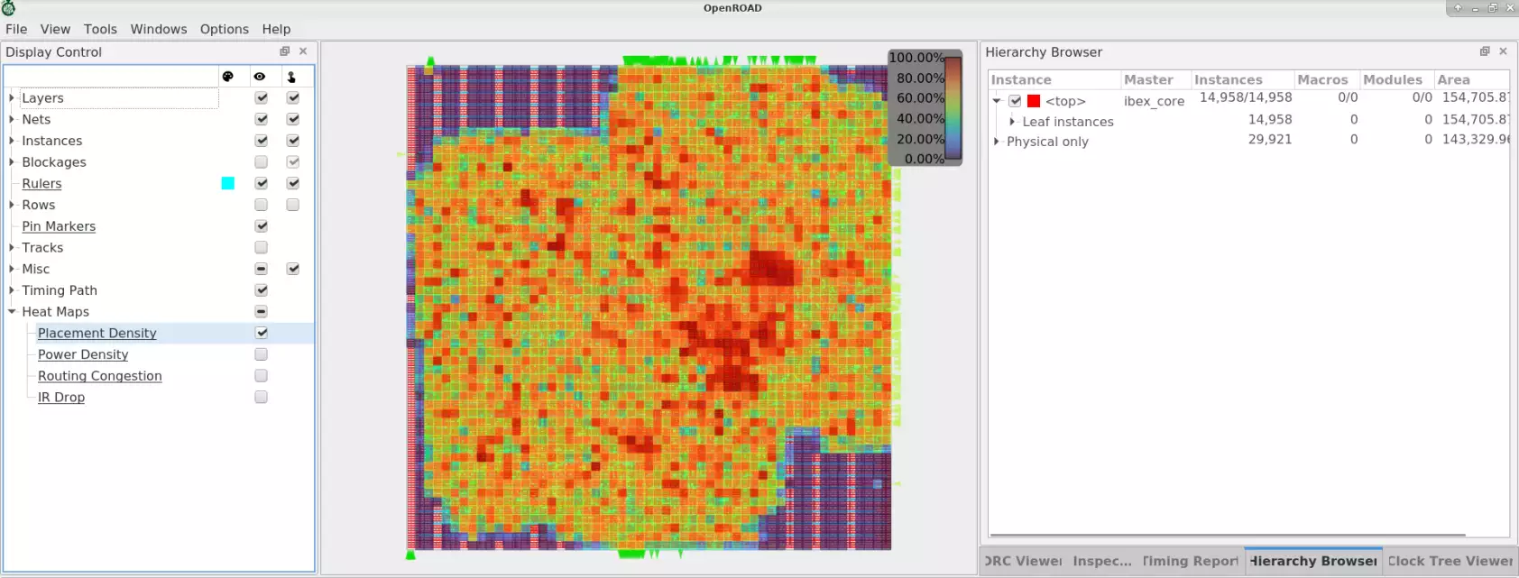
Using Heat Maps#

From the Menu Bar, Click on Tools -> Heat Maps -> Placement Density to view congestion selectively on vertical and horizontal layers.

Expand Heat Maps -> Placement Density from the Display Control window available on LHS of OpenROAD GUI.

View congestion on all layers between 50-100%:

In the Placement density setup pop-up window, Select Minimum -> 50.00% Maximum -> 100.00%

placement_heat_map

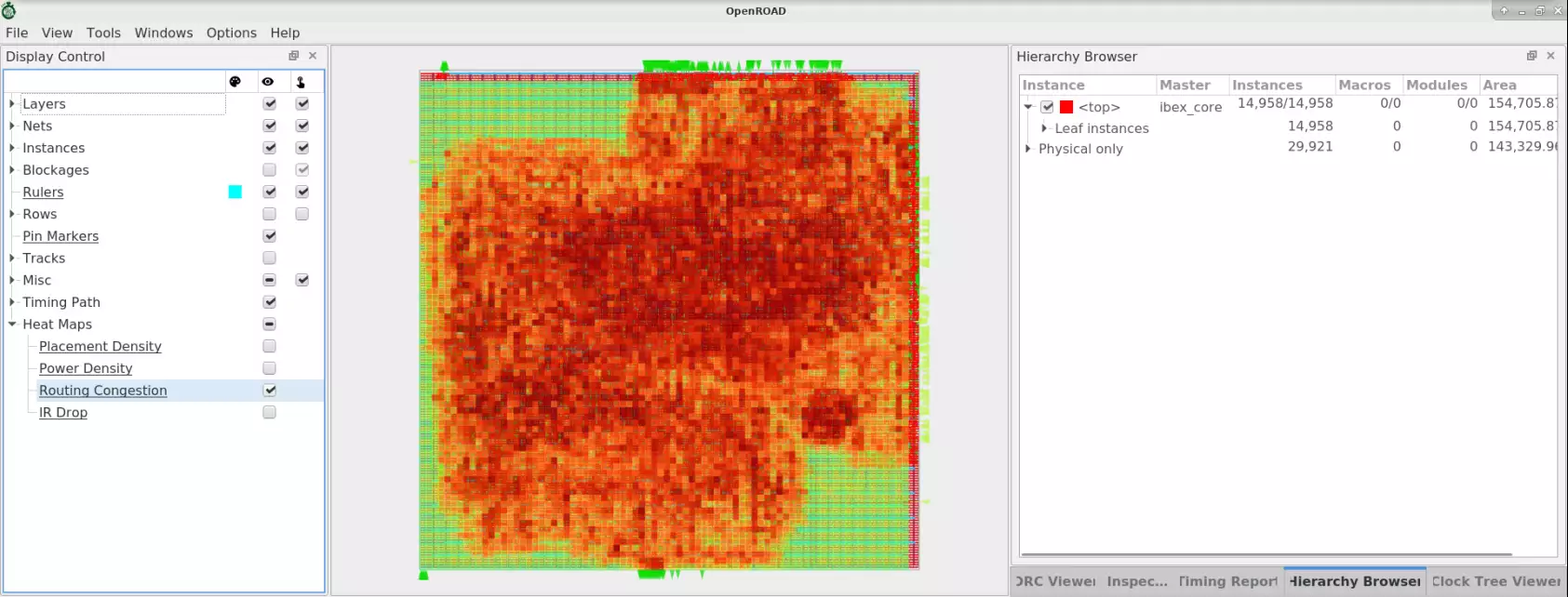
From Display Control, select Heat Maps -> Routing Congestion as follows:

routing_heat_map

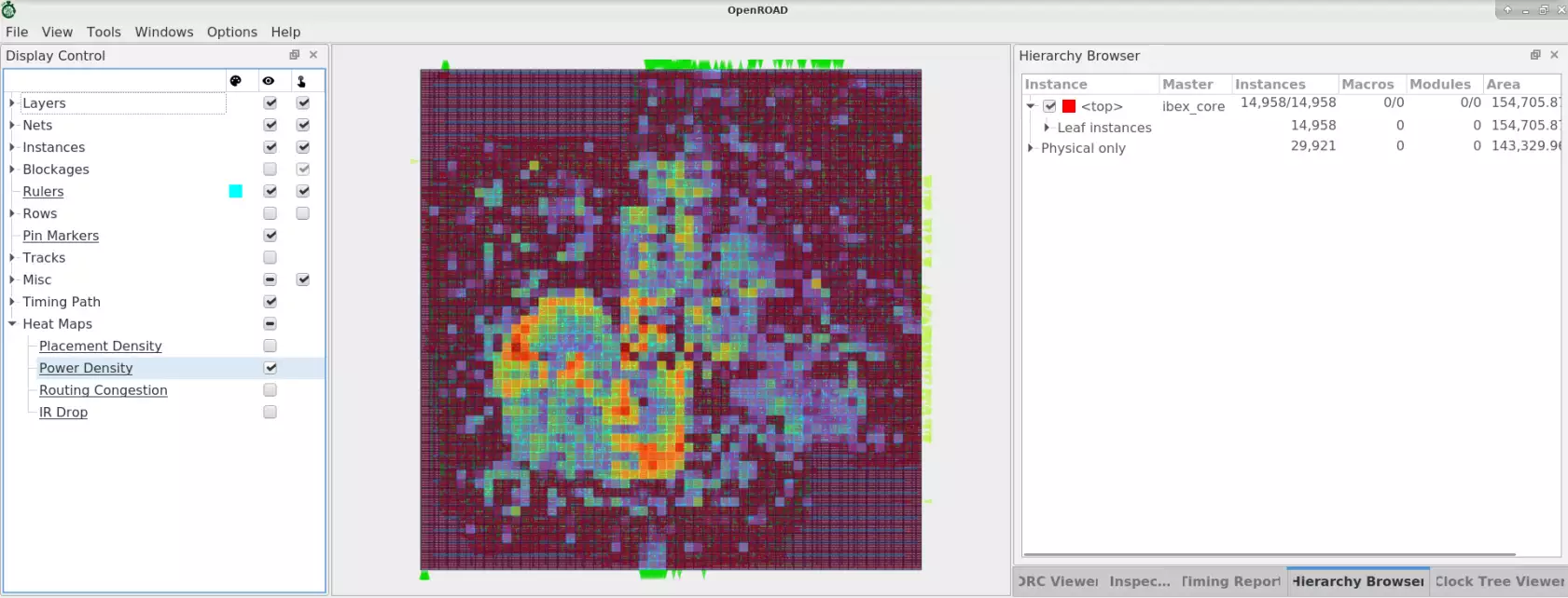
From Display Control, select Heat Maps -> Power Density as follows:

power_heat_map

Viewing Timing Report#

Click Timing -> Options to view and traverse specific timing paths. From Toolbar, click on the Timing icon, View Timing Report window added at the right side (RHS) of GUI as shown below.

Timing report option

In Timing Report Select Paths -> Update, Paths should be integer numbers. The number of timing paths should be displayed in the current window as follows:

Clock Path Update

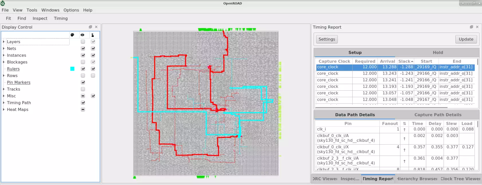
Select Setup or Hold tabs and view required arrival times and slack for each timing path segment.

For each Setup or Hold path group, path details have a specific pin name, Time, Delay, Slew and Load value with the clock to register, register to register and register to output data path.

Using Rulers#

A ruler can measure the distance between any two objects in the design or metal layer length and width to be measured, etc.

Example of how to measure the distance between VDD and VSS power grid click on:

Tools -> Ruler K

Ruler Tool

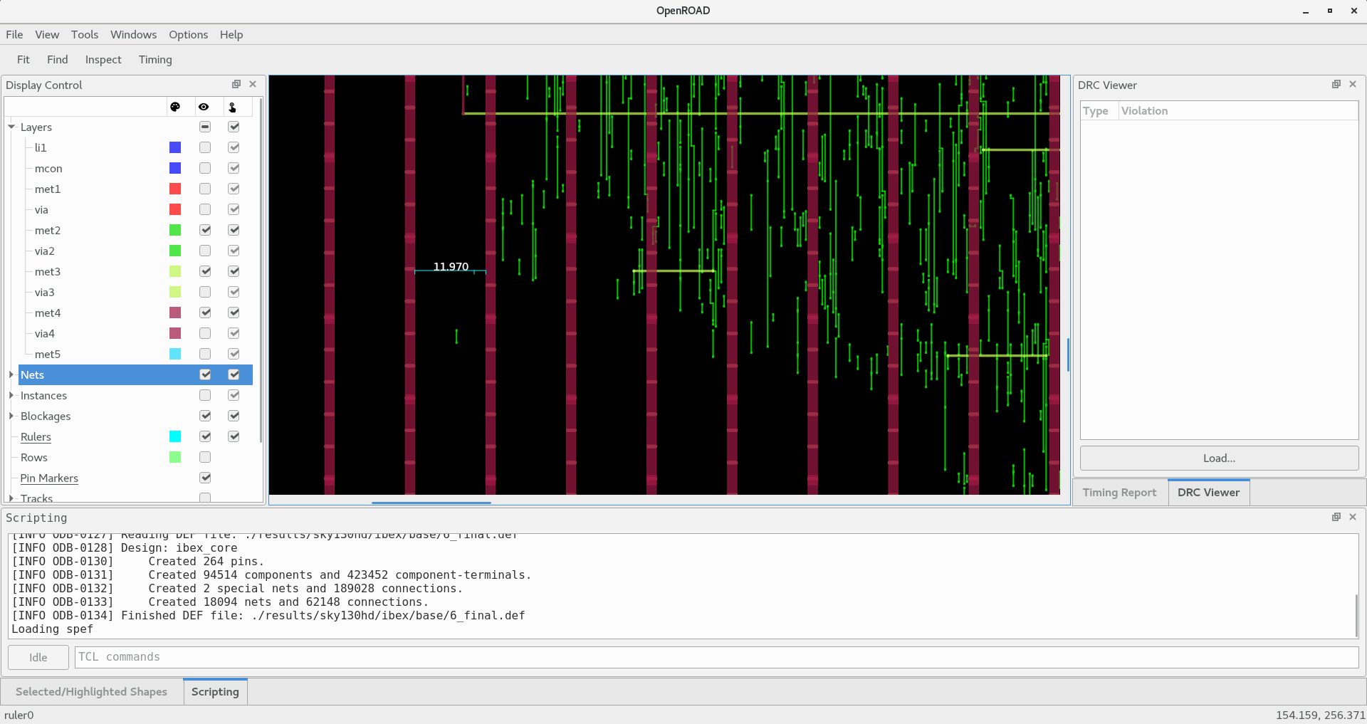
Distance between VDD and VSS layer is 11.970

DRC Viewer#

You can use the GUI to trace DRC violations and fix them.

View DRC violations post routing:

less ./reports/sky130hd/ibex/base/5_route_drc.rpt

Any DRC violations are logged in the 5_route_drc.rpt file, which is empty otherwise.

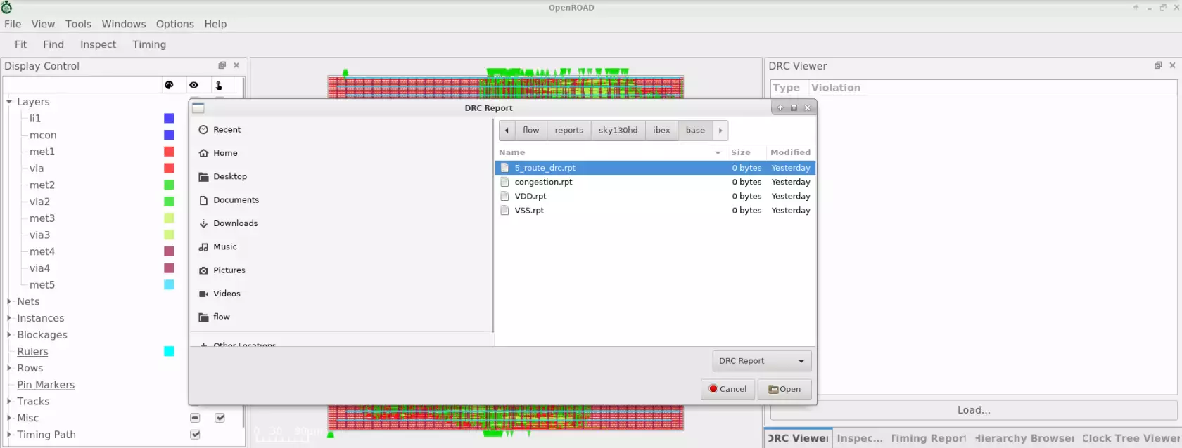
From OpenROAD GUI, Enable the menu options Windows -> DRC Viewer. A DRC viewer window is added on the right side (RHS) of the GUI. From DRC Viewer -> Load navigate to 5_route_drc.rpt

DRC Report Load

By selecting DRC violation details, designers can analyze and fix them. Here user will learn how a DRC violation can be traced with the gcd design. Refer to the following OpenROAD test case for more details.

cd ./flow/tutorials/scripts/drt/
openroad -gui

In the Tcl Commands section of GUI:

source drc_issue.tcl

Post detail routing in the log, you can find the number of violations left in the design:

[INFO DRT-0199] Number of violations = 7.

Based on DRC Viewer steps load results/5_route_drc.rpt. GUI as follows

gcd DRC issue load

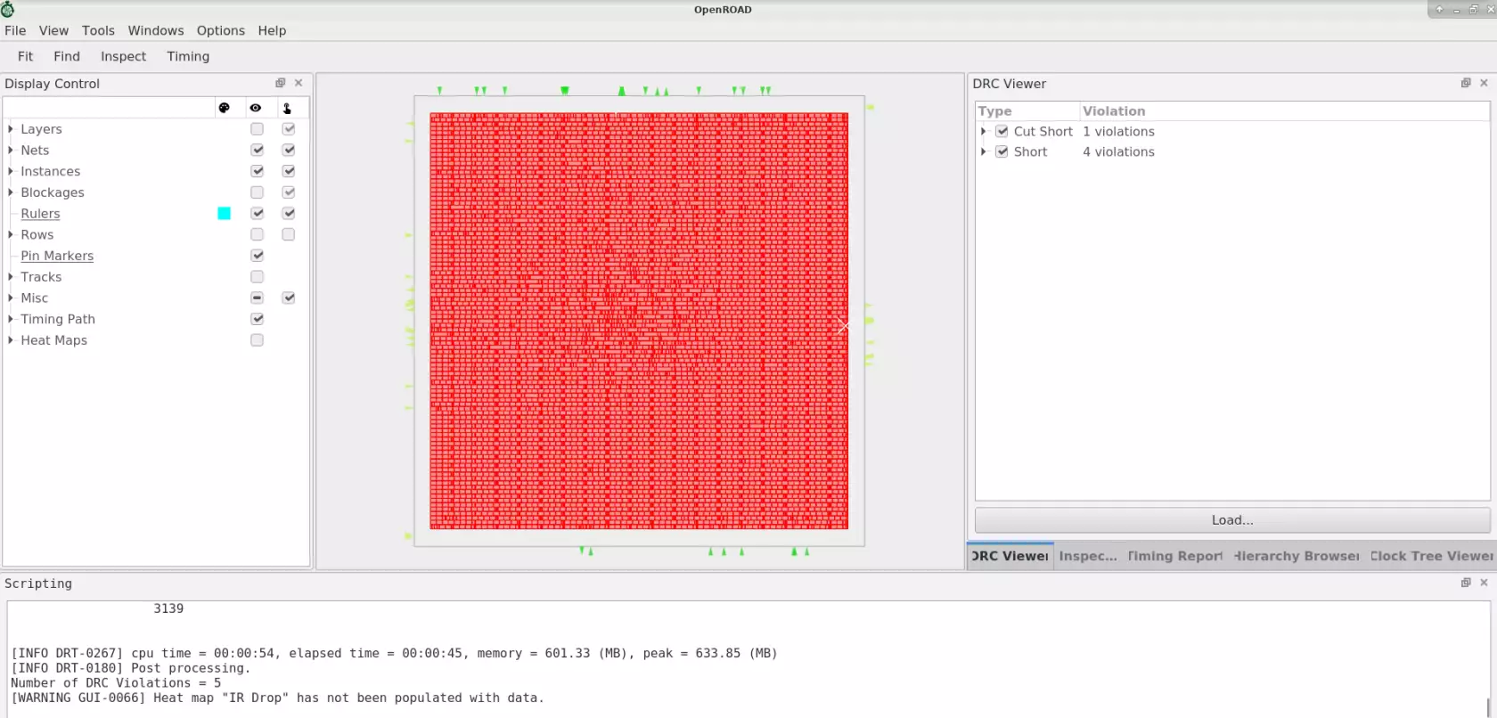
X mark in the design highlights DRC violations.

From DRC Viewer on RHS expand -> Short

This shows the number of violations in the design. Zoom the design for a clean view of the violation:

View DRC Violation

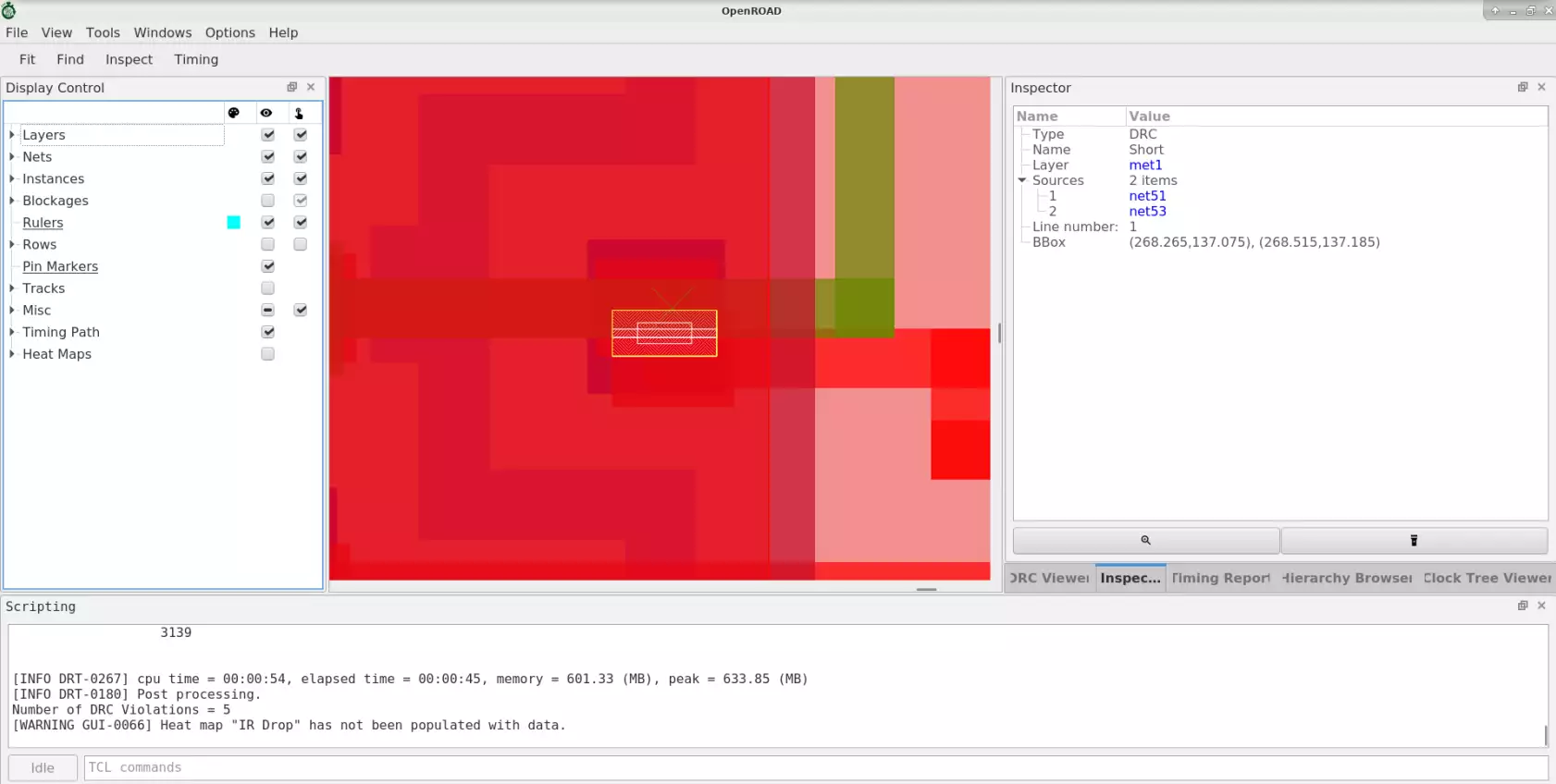
output53 has overlaps and this causes the short violation.

Open the input DEF file drc_cts.def to check the source of the overlap.

Note the snippet of DEF file where output51 and output53 have the same placed coordinates and hence cause the placement violation.

- output51 sky130_fd_sc_hd__clkbuf_1 + PLACED ( 267260 136000 ) N ;
- output53 sky130_fd_sc_hd__clkbuf_1 + PLACED ( 267260 136000 ) N ;

Use the test case provided in 4_cts.def with the changes applied for updated coordinates as follows:

- output51 sky130_fd_sc_hd__clkbuf_1 + PLACED ( 267260 136000 ) N ;
- output53 sky130_fd_sc_hd__clkbuf_1 + PLACED ( 124660 266560 ) N ;

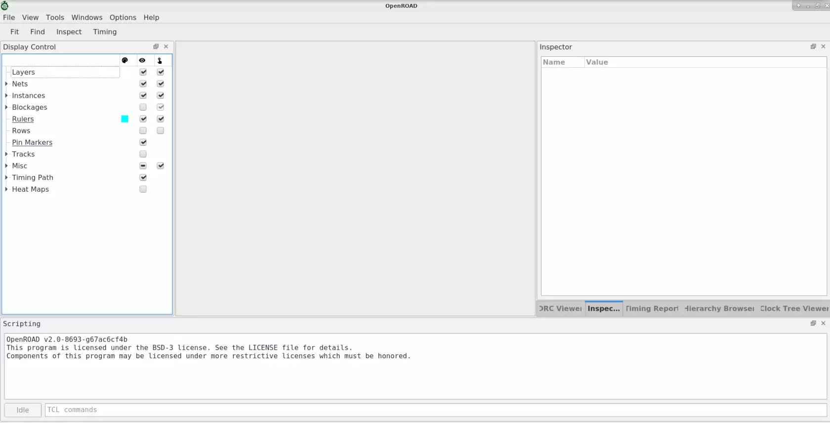
Close the current GUI and re-load the GUI with the updated DEF to see fixed DRC violation in the design:

openroad -gui
source drc_fix.tcl

In the post detail routing log, the user can find the number of violations left in the design:

[INFO DRT-0199] Number of violations = 0.

Routing completed with 0 violations.

Tcl Command Interface#

Execute OpenROAD-flow-scripts Tcl commands from the GUI. Type help to view Tcl Commands available. In OpenROAD GUI, at the bottom, TCL commands executable space is available to run the commands. For example

View design area:

report_design_area

Try the below timing report commands to view timing results interactively:

report_wns
report_tns
report_worst_slack

Customizing The GUI#

Customize the GUI by creating your own widgets such as menu bars, toolbar buttons, dialog boxes, etc.

Refer to the GUI.

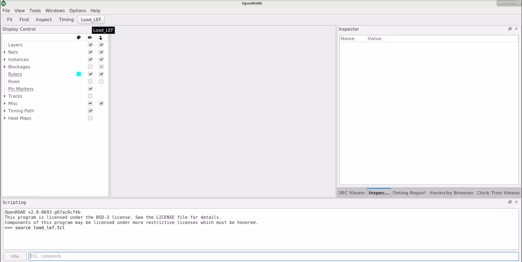
Create Load_LEF toolbar button in GUI to automatically load specified .lef files.

openroad -gui

Default GUI

To view load_lef.tcl, run the command:

less ./flow/tutorials/scripts/gui/load_lef.tcl

proc load_lef_sky130 {} {
    set FLOW_PATH [exec pwd]
    read_lef $FLOW_PATH/../../../platforms/sky130hd/lef/sky130_fd_sc_hd.tlef
    read_lef $FLOW_PATH/../../../platforms/sky130hd/lef/sky130_fd_sc_hd_merged.lef
}
create_toolbar_button -name "Load_LEF" -text "Load_LEF" -script {load_lef_sky130} -echo

From OpenROAD GUI Tcl commands:

cd ./flow/tutorials/scripts/gui/
source load_lef.tcl

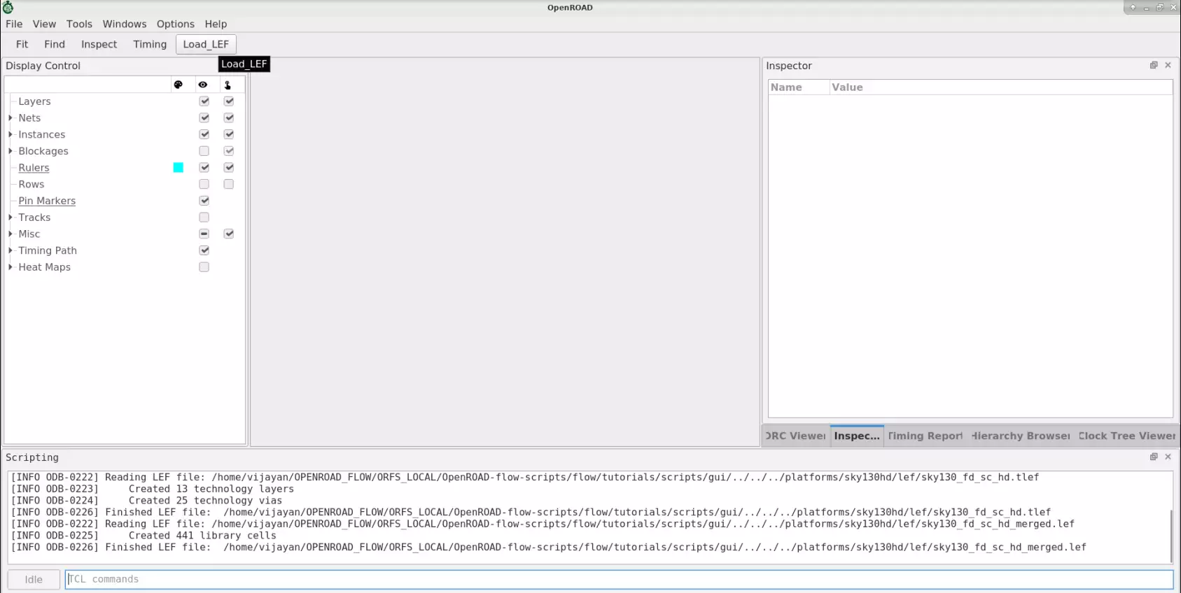
Load_LEF toolbar button added as follows:

Load LEF toolbar button

From Toolbar menus, Click on Load_LEF. This loads the specified sky130 technology .tlef and merged.lef file in the current OpenROAD GUI as follows:

sky130 LEF file load

Understanding and Analyzing OpenROAD Flow Stages and Results#

The OpenROAD flow is fully automated and yet the user can usefully intervene to explore, analyze and optimize your design flow for good PPA.

In this section, you will learn specific details of flow stages and learn to explore various design configurations and optimizations to target specific design goals, i.e., PPA (area, timing, power).

Synthesis Explorations#

Area And Timing Optimization#

Explore optimization options using synthesis options: ABC_AREA and ABC_SPEED.

Set ABC_AREA=1 for area optimization and ABC_SPEED=1 for timing optimization. Update design config.mk for each case and re-run the flow to view impact.

To view ibex design config.mk.

#Synthesis strategies
export ABC_AREA = 1

Run make command from flow directory as follows:

make DESIGN_CONFIG=./designs/sky130hd/gcd/config.mk

The gcd design synthesis results for area and speed optimizations are shown below:

Synthesis Statistics	ABC_SPEED	ABC_AREA
`Number of wires`	224	224
`Number of wire bits`	270	270
`Number of cells`	234	234
`Chip area`	2083.248000	2083.248000
`Final Design Area`	Design area 4295 u^2 6% utilization.	Design area 4074 u^2 6% utilization.

Note: Results for area optimization should be ideally checked after floorplanning to verify the final impact. First, relax the .sdc constraint and re-run to see area impact. Otherwise, the repair design command will increase the area to meet timing regardless of the netlist produced earlier.

Floorplanning#

This section describes OpenROAD-flow-scripts floorplanning and placement functions using the GUI.

Floorplan Initialization Based On Core And Die Area#

Refer to the following OpenROAD built-in examples here.

Run the following commands in the terminal in OpenROAD tool root directory to build and view the created floorplan.

cd ../tools/OpenROAD/src/ifp/test/
openroad -gui

In Tcl Commands section GUI:

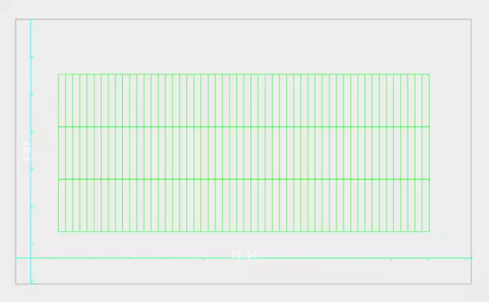
source init_floorplan1.tcl

View the resulting die area “0 0 1000 1000” and core area “100 100 900 900” in microns shown below:

Absolute Floorplan

Floorplan Based On Core Utilization#

Refer to the following OpenROAD built-in examples here.

Run the following commands in the terminal in OpenROAD tool root directory to view how the floorplan initialized:

cd ../tools/OpenROAD/src/ifp/test/
openroad -gui

In the Tcl Commands section of the GUI:

source init_floorplan2.tcl

View the resulting core utilization of 30 created following floorplan:

Relative Floorplan

IO Pin Placement#

Place pins on the boundary of the die on the track grid to minimize net wirelengths. Pin placement also creates a metal shape for each pin using min-area rules.

For designs with unplaced cells, the net wirelength is computed considering the center of the die area as the unplaced cells position.

Find pin placement document here.

Refer to the built-in examples here.

Launch openroad GUI by running the following command(s) in the terminal in OpenROAD tool root directory:

cd ../tools/OpenROAD/src/ppl/test/
openroad -gui

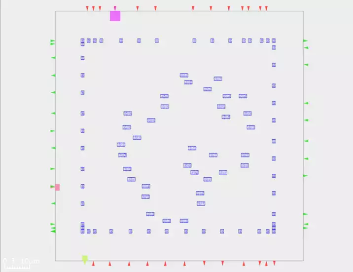
Run place_pin4.tcl script to view pin placement.

From the GUI Tcl commands section:

source place_pin4.tcl

View the resulting pin placement in GUI:

place_pin

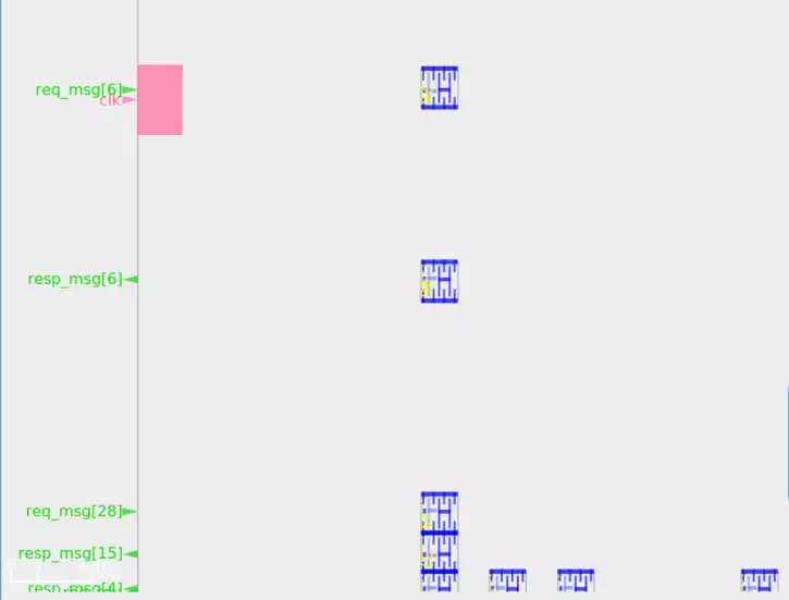
In OpenROAD GUI to enlarge clk pin placement, hold mouse right button as follows and draw sqaure box in specific location:

pin_zoom

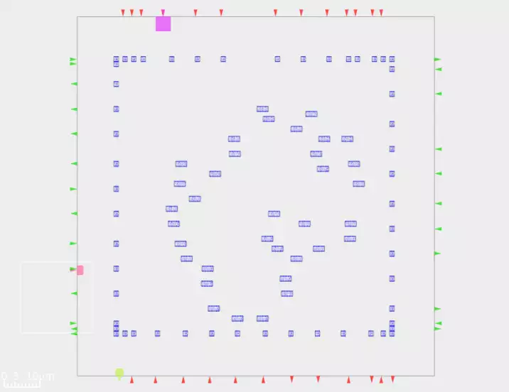
Now clk pin zoom to clear view as follows:

pin_zoomed

Chip Level IO Pad Placement#

In this section, you will generate an I/O pad ring for the coyote design using a Tcl script.

ICeWall is a utility to place IO cells around the periphery of a design, and associate the IO cells with those present in the netlist of the design.

For I/O pad placement using ICeWall refer to the readme file here.

Refer to the built-in examples here.

Launch openroad GUI by running the following command(s) in the terminal in OpenROAD tool root directory:

cd ../tools/OpenROAD/src/pad/test/
openroad -gui

Run skywater130_coyote_tc.tcl script to view IO pad placement.

From the GUI Tcl commands section:

source skywater130_coyote_tc.tcl

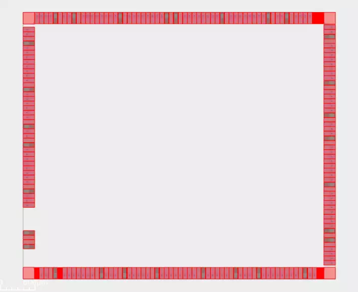
View the resulting IO pad ring in GUI:

coyote pad ring

Power Planning And Analysis#

In this section, you will use the design gcd to create a power grid and run power analysis.

Pdngen is used for power planning. Find the document here.

Refer to the built-in examples here.

Launch openroad GUI by running the following command(s) in the terminal in OpenROAD tool root directory:

cd ../tools/OpenROAD/src/pdn/test
openroad -gui

Run [core_grid_snap.tcl](.(https://github.com/The-OpenROAD-Project/OpenROAD/blob/master/src/pdn/test/core_grid_snap.tcl) to generate power grid for gcd design.

source core_grid_snap.tcl

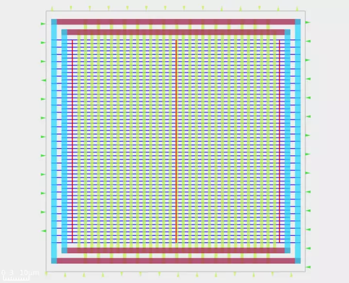
View the resulting power plan for gcd design:

gcd PDN GUI

IR Drop Analysis#

IR drop is the voltage drop in the metal wires constituting the power grid before it reaches the power pins of the standard cells. It becomes very important to limit the IR drop as it affects the speed of the cells and overall performance of the chip.

PDNSim is an open-source static IR analyzer.

Features:

Report worst IR drop.
Report worst current density over all nodes and wire segments in the power distribution network, given a placed and PDN-synthesized design.
Check for floating PDN stripes on the power and ground nets.
Spice netlist writer for power distribution network wire segments.

Refer to the built-in examples here.

Launch openroad by running the following command(s) in the terminal in OpenROAD tool root directory:

cd ../tools/OpenROAD/src/psm/test
openroad

Run gcd_test_vdd.tcl to generate IR drop report for gcd design.

source gcd_test_vdd.tcl

Find the IR drop report at the end of the log as follows:

########## IR report #################
Worstcase voltage: 1.10e+00 V
Average IR drop  : 1.68e-04 V
Worstcase IR drop: 2.98e-04 V
######################################

Tapcell insertion#

Tap cells are non-functional cells that can have a well tie, substrate tie or both. They are typically used when most or all of the standard cells in the library contain no substrate or well taps. Tap cells help tie the VDD and GND levels and thereby prevent drift and latch-up.

The end cap cell or boundary cell is placed at both the ends of each placement row to terminate the row. They protect the standard cell gate at the boundary from damage during manufacturing.

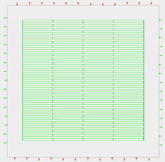
Tap cells are placed after the macro placement and power rail creation. This stage is called the pre-placement stage. Tap cells are placed in a regular interval in each row of placement. The maximum distance between the tap cells must be as per the DRC rule of that particular technology library.

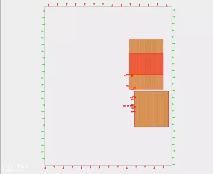
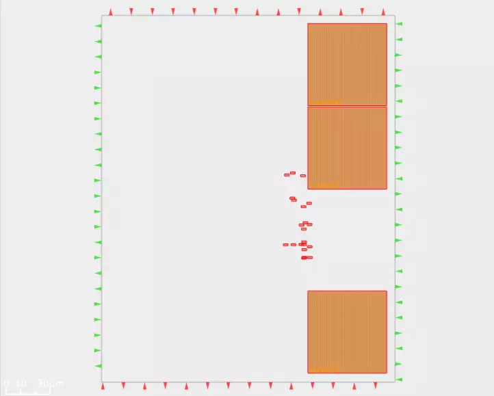
The figures below show two examples of tapcell insertion. When only the -tapcell_master and -endcap_master masters are given, the tapcell placement is similar to Figure 1. When the remaining masters are give, the tapcell placement is similar to Figure 2.

Refer to the GUI figures to highlight well tap and end cap cells. The image does not differentiate and just shows a bunch of rectangles.


Figure 1: Tapcell insertion representation	Figure 2: Tapcell insertion around macro representation

Refer to the following built-in example here to learn about Tap/endcap cell insertion.

To view this in OpenROAD GUI by running the following command(s) in the terminal in OpenROAD tool root directory:

cd ../tools/OpenROAD/src/tap/test/
openroad -gui

In the Tcl Commands section of GUI

source gcd_nangate45.tcl

View the resulting tap cell insertion as follows:

Tap_Cell_Insertion

Tie Cells#

The tie cell is a standard cell, designed specially to provide the high or low signal to the input (gate terminal) of any logic gate. Where ever netlist is having any pin connected to 0 logic or 1 logic (like .A(1’b0) or .IN(1’b1), a tie cell gets inserted there.

Refer to the following built-in example here to learn about Tie cell insertion.

To check this in OpenROAD tool root directory:

cd ../tools/OpenROAD/src/ifp/test/
openroad
source tiecells.tcl

Refer the following verilog code which have tie high/low net. here

AND2_X1 u2 (.A1(r1q), .A2(1'b0), .ZN(u2z0));
AND2_X1 u3 (.A1(u1z), .A2(1'b1), .ZN(u2z1));

With following insert_tiecells command:

insert_tiecells LOGIC0_X1/Z -prefix "TIE_ZERO_"
insert_tiecells LOGIC1_X1/Z

During floorplan stage, those nets converted to tiecells as follows based on library(This is Nangate45 specific):

[INFO IFP-0030] Inserted 1 tiecells using LOGIC0_X1/Z.
[INFO IFP-0030] Inserted 1 tiecells using LOGIC1_X1/Z.

Macro or Standard Cell Placement#

Macro Placement#

In this section, you will explore various placement options for macros and standard cells and study the impact on area and timing.

Refer to the following built-in example here to learn about macro placement.

Placement density impacts how widely standard cells are placed in the core area. To view this in OpenROAD GUI run the following command(s) in the terminal in OpenROAD tool root directory:

cd ../tools/OpenROAD/src/gpl/test/
openroad -gui

In the Tcl Commands section of GUI

source macro01.tcl

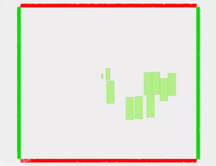
Read the resulting macro placement with a complete core view:


Figure 1: With density 0.7	Figure 2: Zoomed view of macro and std cell placement

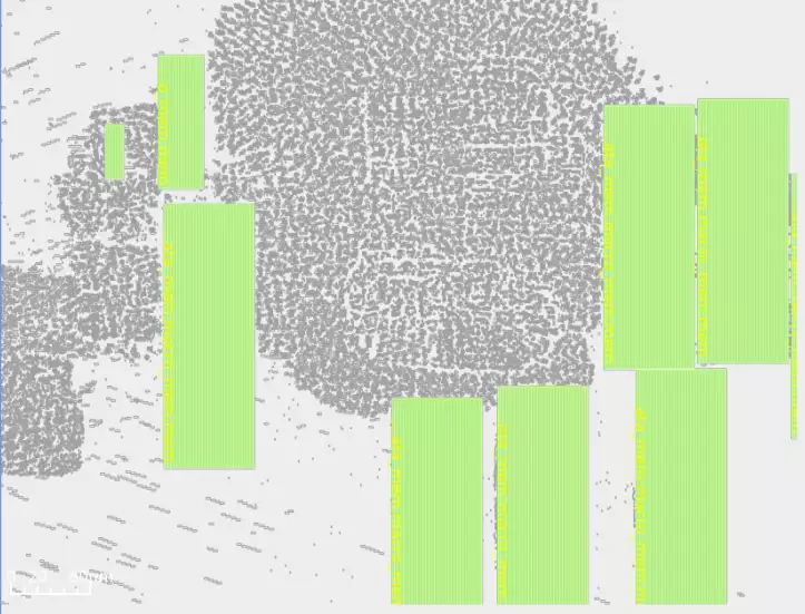
Reduce the placement density and observe the impact on placement, by running below command in Tcl Commands section of GUI:

global_placement -density 0.6

Read the resulting macro placement with a complete core view:


Figure 1: With density 0.6	Figure 2: Zoomed view of macro and std cell placement

Macro Placement With Halo Spacing#

Explore macro placement with halo spacing, refer to the example [here]((https://github.com/The-OpenROAD-Project/OpenROAD/tree/master/src/mpl/test/).

Launch GUI by running the following command(s) in the terminal in OpenROAD tool root directory:

cd ../tools/OpenROAD/src/mpl/test
openroad -gui

In the Tcl Commands section of GUI:

source helpers.tcl
source level3.tcl
global_placement

DEF file without halo spacing

gcd without halo spacing

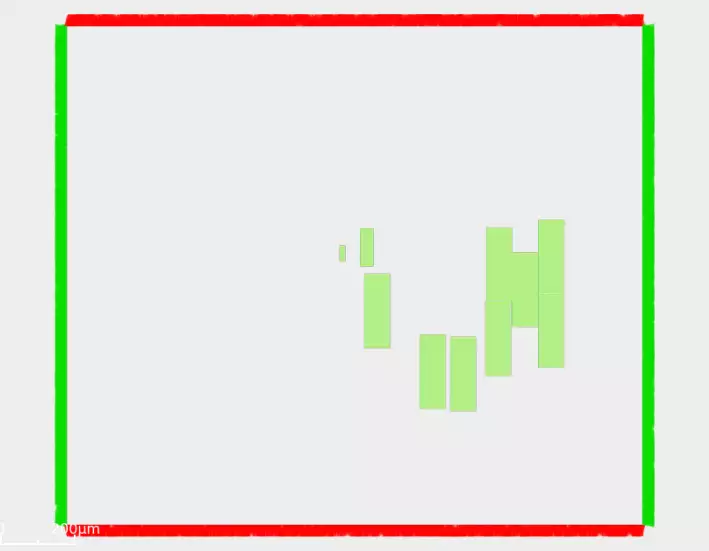
Now increase the halo width for better routing resources.

In the Tcl Commands section of GUI:

macro_placement -halo {0.5 0.5}

Overlapping macros placed 0.5 micron H/V halo around macros.

gcd with halo spacing

Defining Placement Density#

To learn on placement density strategies for ibex design, go to OpenROAD-flow-scripts/flow. Type:

openroad -gui

Enter the following commands in the Tcl Commands section of GUI

read_lef ./platforms/sky130hd/lef/sky130_fd_sc_hd.tlef
read_lef ./platforms/sky130hd/lef/sky130_fd_sc_hd_merged.lef
read_def ./results/sky130hd/ibex/base/3_place.def

ibex placement density 60

Change CORE_UTILIZATION and PLACE_DENSITY for the ibex design config.mk as follows.

View ibex design config.mk here.

export CORE_UTILIZATION = 40
export PLACE_DENSITY_LB_ADDON = 0.1

Re-run the ibex design with the below command:

make DESIGN_CONFIG=./designs/sky130hd/ibex/config.mk

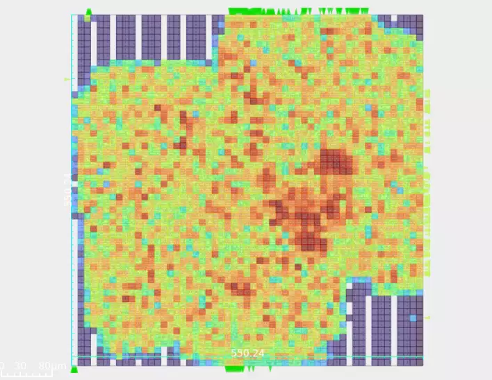
View the ibex design placement density heat map as shown below:

ibex placement density 50

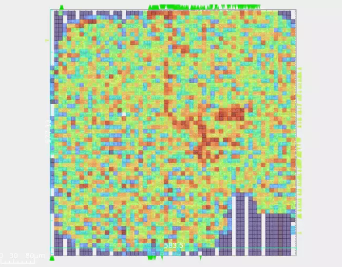
So from above, GUI understood that change in CORE_UTILIZATION from 20 to 40 and placement density default 0.60 to 0.50 changes standard cell placement became widely spread.

Timing Optimizations#

Timing Optimization Using repair_design#

The repair_design command inserts buffers on nets to repair max slew, max capacitance and max fanout violations and on long wires to reduce RC delay. It also resizes gates to normalize slews. Use estimate_parasitics -placement before repair_design to account for estimated post-placement parasitics.

Refer to the built-in example here.

Launch GUI by running the following command(s) in the terminal in OpenROAD tool root directory:

cd ../tools/OpenROAD/src/rsz/test/
openroad -gui

Copy and paste the below commands in the Tcl Commands section of GUI.

source "helpers.tcl"
source "hi_fanout.tcl"
read_liberty Nangate45/Nangate45_typ.lib
read_lef Nangate45/Nangate45.lef
set def_file [make_result_file "repair_slew1.def"]
write_hi_fanout_def $def_file 30
read_def $def_file

create_clock -period 1 clk1
set_wire_rc -layer metal3

estimate_parasitics -placement
set_max_transition .05 [current_design]

puts "Found [sta::max_slew_violation_count] violations"

The number of violations log as:

Found 31 violations

These violations were fixed by:

repair_design

The log is as follows:

[INFO RSZ-0058] Using max wire length 853um.
[INFO RSZ-0039] Resized 1 instance.

To view violation counts again:

puts "Found [sta::max_slew_violation_count] violations"

The log follows:

Found 0 violations

repair_design fixed all 31 violations.

Timing Optimization Using repair_timing#

The repair_timing command repairs setup and hold violations. It was run after clock tree synthesis with propagated clocks.

While repairing hold violations, buffers are not inserted since that may cause setup violations unless ‘-allow_setup_violations’ is specified. Use -slack_margin to add additional slack margin.

Timing Optimization Based On Multiple Corners#

OpenROAD supports multiple corner analysis to calculate worst-case setup and hold violations.

Setup time optimization is based on the slow corner or the best case when the launch clock arrives later than the data clock. Hold time optimization is based on the fast corner or the best case when the launch clock arrives earlier than the capture clock.

Refer to the following gcd design on repair_timing with fast and slow corners.

Refer to the built-in example here.

Run the following commands in the terminal:

cd ../../test/
openroad
source gcd_sky130hd_fast_slow.tcl

The resulting worst slack, TNS:

report_worst_slack -min -digits 3
worst slack 0.321
report_worst_slack -max -digits 3
worst slack -16.005
report_tns -digits 3
tns -529.496

Fixing Setup Violations#

To fix setup timing path violations, use repair_timing -setup.

Refer to the following built-in example to learn more about fixing setup timing violations.

Refer to the built-in example here.

Launch OpenROAD in an interactive mode by running the following command(s) in the terminal in OpenROAD tool root directory:

cd ../tools/OpenROAD/src/rsz/test/
openroad

Copy and paste the following Tcl commands.

define_corners fast slow
read_liberty -corner slow Nangate45/Nangate45_slow.lib
read_liberty -corner fast Nangate45/Nangate45_fast.lib
read_lef Nangate45/Nangate45.lef
read_def repair_setup1.def
create_clock -period 0.3 clk
set_wire_rc -layer metal3
estimate_parasitics -placement
report_checks -fields input -digits 3

View the generated timing report with the slack violation.

Startpoint: r1 (rising edge-triggered flip-flop clocked by clk)
Endpoint: r2 (rising edge-triggered flip-flop clocked by clk)
Path Group: clk
Path Type: max
Corner: slow

   Delay     Time   Description
-----------------------------------------------------------
   0.000    0.000   clock clk (rise edge)
   0.000    0.000   clock network delay (ideal)
   0.000    0.000 ^ r1/CK (DFF_X1)
   0.835    0.835 ^ r1/Q (DFF_X1)
   0.001    0.836 ^ u1/A (BUF_X1)
   0.196    1.032 ^ u1/Z (BUF_X1)
   0.001    1.033 ^ u2/A (BUF_X1)
   0.121    1.154 ^ u2/Z (BUF_X1)
   0.001    1.155 ^ u3/A (BUF_X1)
   0.118    1.273 ^ u3/Z (BUF_X1)
   0.001    1.275 ^ u4/A (BUF_X1)
   0.118    1.393 ^ u4/Z (BUF_X1)
   0.001    1.394 ^ u5/A (BUF_X1)
   0.367    1.761 ^ u5/Z (BUF_X1)
   0.048    1.809 ^ r2/D (DFF_X1)
            1.809   data arrival time

   0.300    0.300   clock clk (rise edge)
   0.000    0.300   clock network delay (ideal)
   0.000    0.300   clock reconvergence pessimism
            0.300 ^ r2/CK (DFF_X1)
  -0.155    0.145   library setup time
            0.145   data required time
-----------------------------------------------------------
            0.145   data required time
           -1.809   data arrival time
-----------------------------------------------------------
           -1.664   slack (VIOLATED)

Fix setup violation using:

repair_timing -setup

The log is as follows:

[INFO RSZ-0040] Inserted 4 buffers.
[INFO RSZ-0041] Resized 16 instances.
[WARNING RSZ-0062] Unable to repair all setup violations.

Reduce the clock frequency by increasing the clock period to 0.9 and re-run repair_timing to fix the setup violation warnings. Such timing violations are automatically fixed by the resizer post CTS and global routing.

create_clock -period 0.9 clk
repair_timing -setup

To view timing logs post-repair timing, type:

report_checks -fields input -digits 3

The log is as follows:

Startpoint: r1 (rising edge-triggered flip-flop clocked by clk)
Endpoint: r2 (rising edge-triggered flip-flop clocked by clk)
Path Group: clk
Path Type: max
Corner: slow

   Delay     Time   Description
-----------------------------------------------------------
   0.000    0.000   clock clk (rise edge)
   0.000    0.000   clock network delay (ideal)
   0.000    0.000 ^ r1/CK (DFF_X1)
   0.264    0.264 v r1/Q (DFF_X1)
   0.002    0.266 v u1/A (BUF_X4)
   0.090    0.356 v u1/Z (BUF_X4)
   0.003    0.359 v u2/A (BUF_X8)
   0.076    0.435 v u2/Z (BUF_X8)
   0.003    0.438 v u3/A (BUF_X8)
   0.074    0.512 v u3/Z (BUF_X8)
   0.003    0.515 v u4/A (BUF_X8)
   0.077    0.592 v u4/Z (BUF_X8)
   0.005    0.597 v u5/A (BUF_X16)
   0.077    0.674 v u5/Z (BUF_X16)
   0.036    0.710 v r2/D (DFF_X1)
            0.710   data arrival time

   0.900    0.900   clock clk (rise edge)
   0.000    0.900   clock network delay (ideal)
   0.000    0.900   clock reconvergence pessimism
            0.900 ^ r2/CK (DFF_X1)
  -0.172    0.728   library setup time
            0.728   data required time
-----------------------------------------------------------
            0.728   data required time
           -0.710   data arrival time
-----------------------------------------------------------
            0.019   slack (MET)

Fixing Hold Violations#

To fix hold violation for the design, command to use repair_timing -hold

Refer to the example here to learn more about fixing hold violations.

Check hold violation post-global routing using the following Tcl commands. Run below steps in terminal in OpenROAD tool root directory:

cd ../tools/OpenROAD/src/rsz/test/
openroad -gui

Copy and paste the below commands in the Tcl Commands section of GUI.

source helpers.tcl
read_liberty sky130hd/sky130hd_tt.lib
read_lef sky130hd/sky130hd.tlef
read_lef sky130hd/sky130hd_std_cell.lef
read_def repair_hold10.def
create_clock -period 2 clk
set_propagated_clock clk
set_wire_rc -resistance 0.0001 -capacitance 0.00001
set_routing_layers -signal met1-met5
global_route
estimate_parasitics -global_routing
report_worst_slack -min

Read the resulting worst slack as:

worst slack -1.95

The above worst slack was fixed with:

repair_timing -hold

The log is as follows:

[INFO RSZ-0046] Found 2 endpoints with hold violations.
[INFO RSZ-0032] Inserted 5 hold buffers.

Re-check the slack value after repair_timing. Type:

report_worst_slack -min

The result worst slack value is as follows:

worst slack 0.16

Note that the worst slack is now met and the hold violation was fixed by the resizer.

Clock Tree Synthesis#

To perform clock tree synthesis clock_tree_synthesis flow command used. The OpenROAD-flow-scripts automatically generates a well-balanced clock tree post-placement. In this section, you will learn details about the building and visualize the clock tree.

Refer to the built-in example here.

Launch OpenROAD GUI by running the following command(s) in the terminal in OpenROAD tool root directory:

cd ../tools/OpenROAD/src/cts/test/
openroad -gui

To build the clock tree, run the following commands in Tcl Commands of GUI:

read_lef Nangate45/Nangate45.lef
read_liberty Nangate45/Nangate45_typ.lib
read_def "16sinks.def"
create_clock -period 5 clk
set_wire_rc -clock -layer metal3
clock_tree_synthesis -root_buf CLKBUF_X3 \
                     -buf_list CLKBUF_X3 \
                     -wire_unit 20

Layout view before CTS as follows:

Layout view after CTS can be viewed with Update option.

Here we explore how clock tree buffers are inserted to balance the clock tree structure.

Refer to the built-in example here.

Generate a clock- tree that is unbalanced first, then explore the creation of a well-balanced clock tree.

Launch OpenROAD GUI by running the following command(s) in the terminal in OpenROAD tool root directory:

cd ../tools/OpenROAD/src/cts/test/
openroad -gui

Use the following commands in the TCL commands section of GUI:

source "helpers.tcl"
source "cts-helpers.tcl"
read_liberty Nangate45/Nangate45_typ.lib
read_lef Nangate45/Nangate45.lef
set block [make_array 300 200000 200000 150]
sta::db_network_defined
create_clock -period 5 clk
set_wire_rc -clock -layer metal5

The clock tree structure is as follows with unbalanced mode.

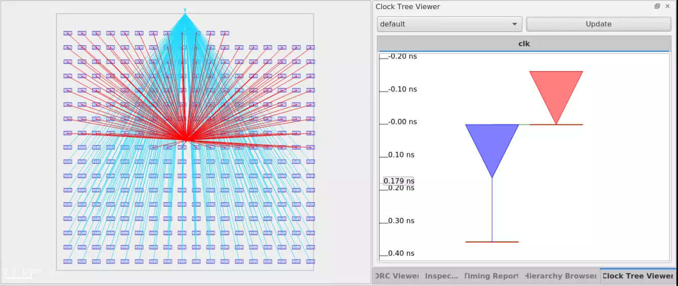
Use the clock_tree_synthesis command to balance this clock tree structure with buffers. See the format as follows.

clock_tree_synthesis -root_buf CLKBUF_X3 \
                     -buf_list CLKBUF_X3 \
                     -wire_unit 20 \
                     -post_cts_disable \
                     -sink_clustering_enable \
                     -distance_between_buffers 100 \
                     -sink_clustering_size 10 \
                     -sink_clustering_max_diameter 60 \
                     -balance_levels \
                     -num_static_layers 1

To view the balanced clock tree after CTS, in GUI Toolbar, select

Clock Tree Viewer and click Update to view the resulting clock tree in GUI as follows:

Reporting Clock Skews#

The OpenROAD-flow-scripts flow automatically fixes any skew issues that could potentially cause hold violations downstream in the timing path.

report_clock_skew

For the ibex design, refer to the following logs to view clock skew reports.

less logs/sky130hd/ibex/base/4_1_cts.log

cts pre-repair report_clock_skew
--------------------------------------------------------------------------
Clock core_clock
Latency      CRPR       Skew
_28453_/CLK ^
   5.92
_29312_/CLK ^
   1.41      0.00       4.51

cts post-repair report_clock_skew
--------------------------------------------------------------------------
Clock core_clock
Latency      CRPR       Skew
_28453_/CLK ^
   5.92
_29312_/CLK ^
   1.41      0.00       4.51

cts final report_clock_skew
--------------------------------------------------------------------------
Clock core_clock
Latency      CRPR       Skew
_27810_/CLK ^
   5.97
_29266_/CLK ^
   1.41      0.00       4.56

Reporting CTS Metrics#

Run report_cts command to view useful metrics such as number of clock roots, number of buffers inserted, number of clock subnets and number of sinks.

Refer to the built-in examples here.

Run these Tcl commands in the terminal in OpenROAD tool root directory:

cd ../tools/OpenROAD/src/cts/test/
openroad
source post_cts_opt.tcl
report_cts

CTS metrics are as follows for the current design.

[INFO CTS-0003] Total number of Clock Roots: 1.
[INFO CTS-0004] Total number of Buffers Inserted: 35.
[INFO CTS-0005] Total number of Clock Subnets: 35.
[INFO CTS-0006] Total number of Sinks: 301.

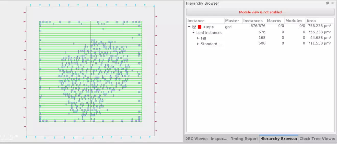
Adding Filler Cells#

Filler cells fills gaps between detail-placed instances to connect the power and ground rails in the rows. Filler cells have no logical connectivity. These cells are provided continuity in the rows for VDD and VSS nets and it also contains substrate nwell connection to improve substrate biasing.

filler_masters is a list of master/macro names to use for filling the gaps.

Refer to the following built-in example here to learn about filler cell insertion.

To view this in OpenROAD GUI run the following command(s) in the terminal in OpenROAD tool root directory:

cd ../tools/OpenROAD/src/grt/test/
openroad -gui

In the Tcl Commands section of GUI,run following commands:

source "helpers.tcl"
read_lef "Nangate45/Nangate45.lef"
read_def "gcd.def"

Loaded DEF view without filler insertion:

Without_Fill_Cell_Insertion

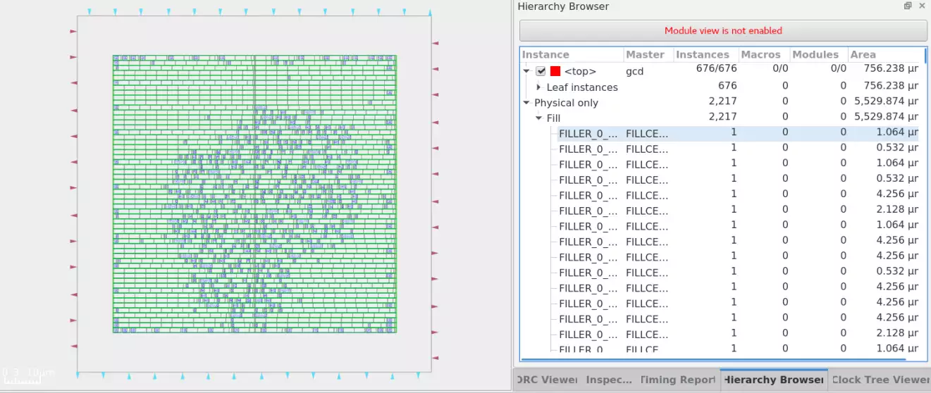
Run following commands for filler cell insertion:

set filler_master [list FILLCELL_X1 FILLCELL_X2 FILLCELL_X4 FILLCELL_X8 FILLCELL_X16]
filler_placement $filler_master

View the resulting fill cell insertion as follows:

Fill_Cell_Insertion

Filler cells removed with remove_fillers command.

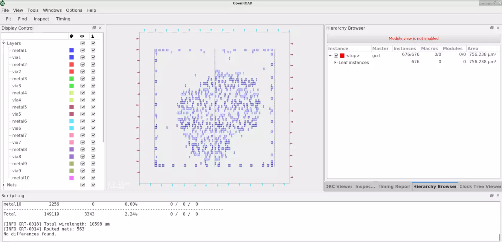
Global Routing#

The global router analyzes available routing resources and automatically allocates them to avoid any H/V overflow violations for optimal routing. It generates a congestion report for GCells showing total resources, demand, utilization, location and the H/V violation status. If there are no violations reported then the design can proceed to detail routing.

Refer to the built-in example here.

Launch OpenROAD GUI by running the following command(s) in the terminal in OpenROAD tool root directory:

cd ../tools/OpenROAD/src/grt/test/
openroad -gui

To run the global routing, run the following commands in Tcl Commands of GUI:

source gcd.tcl

Routing resource and congestion analysis done with below log:

[INFO GRT-0096] Final congestion report:
Layer         Resource        Demand        Usage (%)    Max H / Max V / Total Overflow
---------------------------------------------------------------------------------------
metal1           31235          1651            5.29%             0 /  0 /  0
metal2           24628          1652            6.71%             0 /  0 /  0
metal3           33120            40            0.12%             0 /  0 /  0
metal4           15698             0            0.00%             0 /  0 /  0
metal5           15404             0            0.00%             0 /  0 /  0
metal6           15642             0            0.00%             0 /  0 /  0
metal7            4416             0            0.00%             0 /  0 /  0
metal8            4512             0            0.00%             0 /  0 /  0
metal9            2208             0            0.00%             0 /  0 /  0
metal10           2256             0            0.00%             0 /  0 /  0
---------------------------------------------------------------------------------------
Total           149119          3343            2.24%             0 /  0 /  0

[INFO GRT-0018] Total wirelength: 10598 um
[INFO GRT-0014] Routed nets: 563

View the resulting global routing in GUI as follows:

Global Route

Detail Routing#

TritonRoute is an open-source detailed router for modern industrial designs. The router consists of several main building blocks, including pin access analysis, track assignment, initial detailed routing, search and repair, and a DRC engine.

Refer to the built-in example here.

Launch OpenROAD GUI by running the following command(s) in the terminal in OpenROAD tool root directory:

cd ../tools/OpenROAD/src/drt/test/
openroad -gui

To run the detail routing, run the following commands in Tcl Commands of GUI:

read_lef Nangate45/Nangate45_tech.lef
read_lef Nangate45/Nangate45_stdcell.lef
read_def gcd_nangate45_preroute.def
read_guides gcd_nangate45.route_guide
set_thread_count [expr [exec getconf _NPROCESSORS_ONLN] / 4]
detailed_route -output_drc results/gcd_nangate45.output.drc.rpt \
               -output_maze results/gcd_nangate45.output.maze.log \
               -verbose 1
write_db gcd_nangate45.odb

For successful routing, DRT will end with 0 violations.

Log as follows:

[INFO DRT-0199]   Number of violations = 0.
[INFO DRT-0267] cpu time = 00:00:00, elapsed time = 00:00:00, memory = 674.22 (MB), peak = 686.08 (MB)
Total wire length = 5680 um.
Total wire length on LAYER metal1 = 19 um.
Total wire length on LAYER metal2 = 2798 um.
Total wire length on LAYER metal3 = 2614 um.
Total wire length on LAYER metal4 = 116 um.
Total wire length on LAYER metal5 = 63 um.
Total wire length on LAYER metal6 = 36 um.
Total wire length on LAYER metal7 = 32 um.
Total wire length on LAYER metal8 = 0 um.
Total wire length on LAYER metal9 = 0 um.
Total wire length on LAYER metal10 = 0 um.
Total number of vias = 2223.
Up-via summary (total 2223):.

---------------
 active       0
 metal1    1151
 metal2    1037
 metal3      22
 metal4       7
 metal5       4
 metal6       2
 metal7       0
 metal8       0
 metal9       0
---------------
           2223


[INFO DRT-0198] Complete detail routing.

View the resulting detail routing in GUI as follows:

Detail Routing

Antenna Checker#

Antenna Violation occurs when the antenna ratio exceeds a value specified in a Process Design Kit (PDK). The antenna ratio is the ratio of the gate area to the gate oxide area. The amount of charge collection is determined by the area/size of the conductor (gate area).

This tool checks antenna violations and generates a report to indicate violated nets.

Refer to the built-in example here.

Launch OpenROAD by running the following command(s) in the terminal in OpenROAD tool root directory:

cd ../tools/OpenROAD/src/ant/test/
openroad

To extract antenna violations, run the following commands:

read_lef ant_check.lef
read_def ant_check.def

check_antennas -verbose
puts "violation count = [ant::antenna_violation_count]"

# check if net50 has a violation
set net "net50"
puts "Net $net violations: [ant::check_net_violation $net]"

The log as follows:

[INFO ANT-0002] Found 1 net violations.
[INFO ANT-0001] Found 2 pin violations.
violation count = 1
Net net50 violations: 1

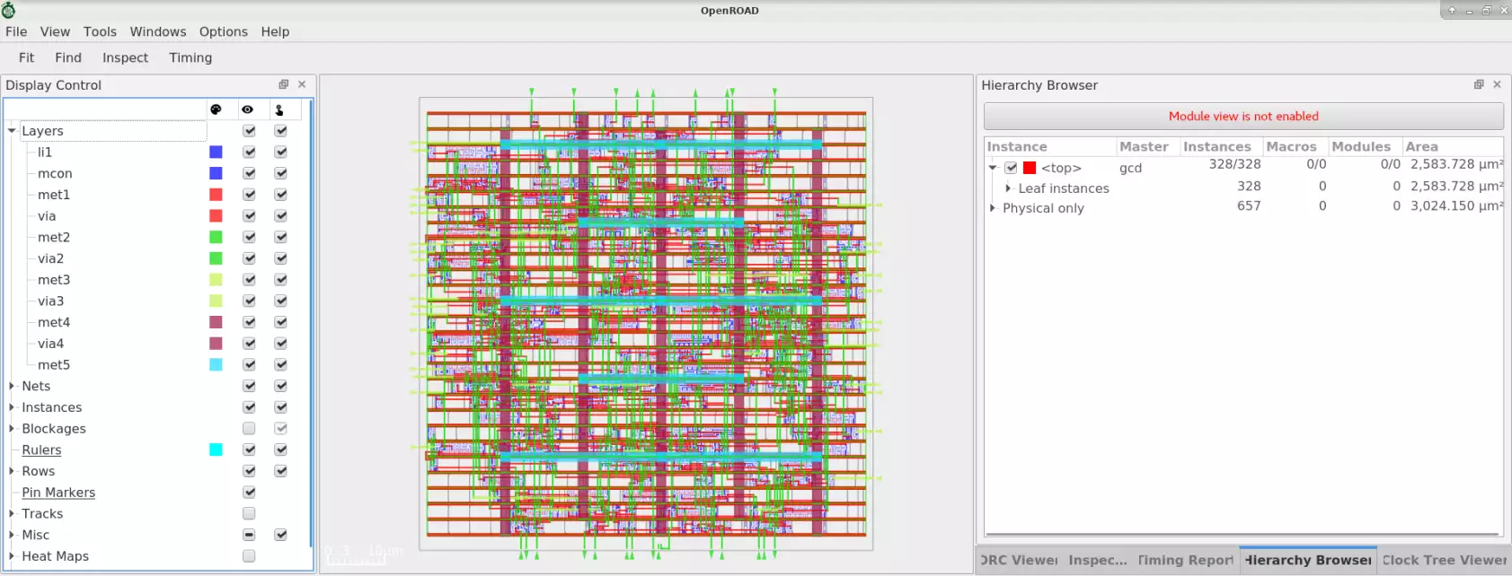
Metal Fill#

Metal fill is a mandatory step at advanced nodes to ensure manufacturability and high yield. It involves filling the empty or white spaces near the design with metal polygons to ensure regular planarization of the wafer.

This module inserts floating metal fill shapes to meet metal density design rules while obeying DRC constraints. It is driven by a json configuration file.

Command used as follows:

density_fill -rules <json_file> [-area <list of lx ly ux uy>]

If -area is not specified, the core area will be used.

To run metal fill post route, run the following:

cd flow/tutorials/scripts/metal_fill
openroad -gui
source "helpers.tcl"
read_db ./5_route.odb

Layout before adding metal fill is as follows: Detail Routing

To add metal fill, run the command:

density_fill -rules ../../../platforms/sky130hd/fill.json

Layout after adding metal fill insertion is as follows:

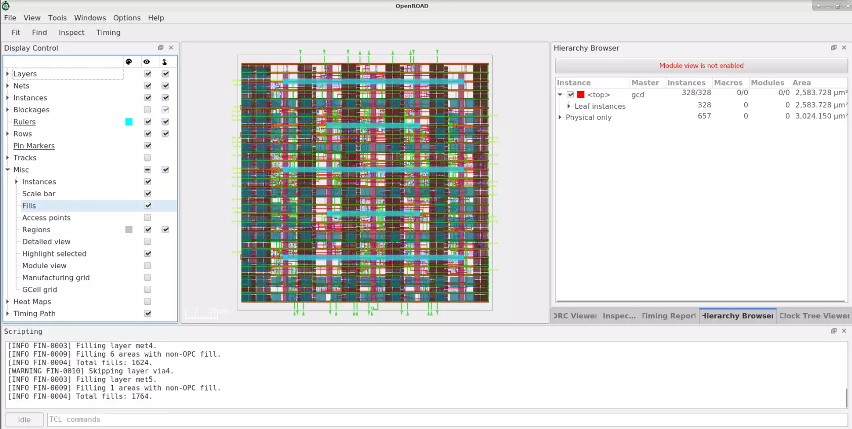
Metal fill view can enabled with Misc and enable Fills check box.

Parasitics Extraction#

OpenRCX is a Parasitic Extraction (PEX, or RCX) tool that works on OpenDB design APIs. It extracts routed designs based on the LEF/DEF layout model.

OpenRCX stores resistance, coupling capacitance and ground (i.e., grounded) capacitance on OpenDB objects with direct pointers to the associated wire and via db objects. Optionally, OpenRCX can generate a .spef file.

Refer to the built-in example here.

Launch OpenROAD tool by running the following command(s) in the terminal in OpenROAD tool root directory:

cd ../tools/OpenROAD/src/rcx/test/
openroad

To run parasitics for gcd design:

source 45_gcd.tcl

The log as follows:

[INFO ODB-0222] Reading LEF file: Nangate45/Nangate45.lef
[INFO ODB-0223]     Created 22 technology layers
[INFO ODB-0224]     Created 27 technology vias
[INFO ODB-0225]     Created 135 library cells
[INFO ODB-0226] Finished LEF file:  Nangate45/Nangate45.lef
[INFO ODB-0127] Reading DEF file: 45_gcd.def
[INFO ODB-0128] Design: gcd
[INFO ODB-0130]     Created 54 pins.
[INFO ODB-0131]     Created 1820 components and 4618 component-terminals.
[INFO ODB-0132]     Created 2 special nets and 3640 connections.
[INFO ODB-0133]     Created 350 nets and 978 connections.
[INFO ODB-0134] Finished DEF file: 45_gcd.def
[INFO RCX-0431] Defined process_corner X with ext_model_index 0
[INFO RCX-0029] Defined extraction corner X
[INFO RCX-0008] extracting parasitics of gcd ...
[INFO RCX-0435] Reading extraction model file 45_patterns.rules ...
[INFO RCX-0436] RC segment generation gcd (max_merge_res 0.0) ...
[INFO RCX-0040] Final 2656 rc segments
[INFO RCX-0439] Coupling Cap extraction gcd ...
[INFO RCX-0440] Coupling threshhold is 0.1000 fF, coupling capacitance less than 0.1000 fF will be grounded.
[INFO RCX-0043] 1954 wires to be extracted
[INFO RCX-0442] 48% completion -- 954 wires have been extracted
[INFO RCX-0442] 100% completion -- 1954 wires have been extracted
[INFO RCX-0045] Extract 350 nets, 2972 rsegs, 2972 caps, 2876 ccs
[INFO RCX-0015] Finished extracting gcd.
[INFO RCX-0016] Writing SPEF ...
[INFO RCX-0443] 350 nets finished
[INFO RCX-0017] Finished writing SPEF ...

45_gcd.spef viewed in results directory.

Troubleshooting Problems#

This section shows you how to troubleshoot commonly occurring problems with the flow or any of the underlying application tools.

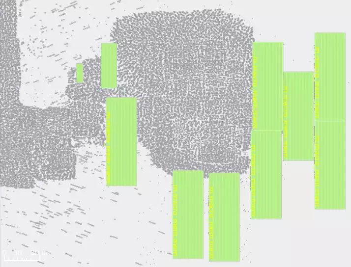
Debugging Problems in Global Routing#

The global router has a few useful functionalities to understand high congestion issues in the designs.

Congestion heatmap can be used on any design, whether it has congestion or not. Viewing congestion explained here. If the design has congestion issue, it ends with the error;

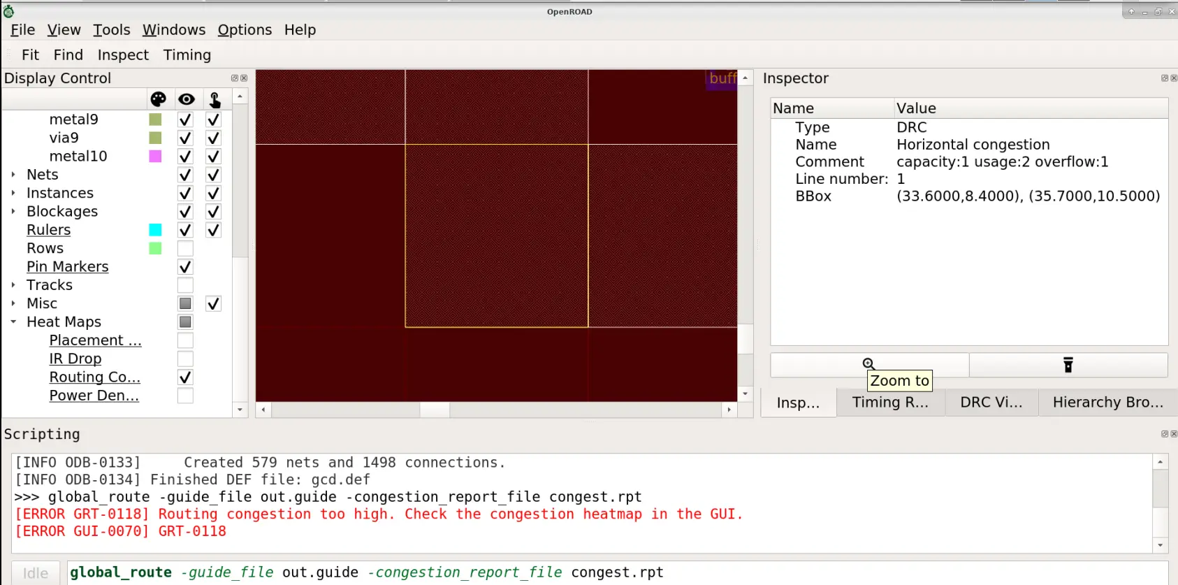
[ERROR GRT-0118] Routing congestion too high.

Refer to the built-in example here.

Launch OpenROAD GUI by running the following command(s) in the terminal in OpenROAD tool root directory:

cd ../tools/OpenROAD/src/grt/test/
openroad -gui

To run the global routing, run the following commands in Tcl Commands of GUI:

source congestion5.tcl

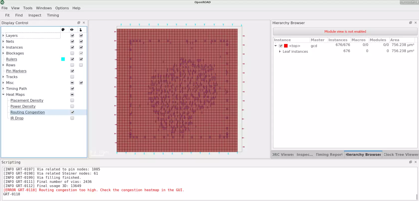
The design fail with routing congestion error as follows: Routing_Congestion

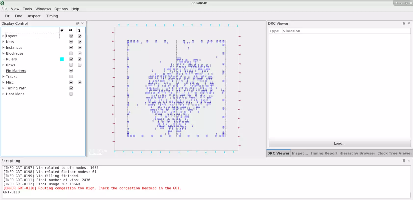
In the GUI, you can go under Heat Maps and mark the Routing Congestion checkbox to visualize the congestion map. congestion_heatmap

Dump congestion information to a text file#

You can create a text file with the congestion information of the GCells for further investigation on the GUI. To do that, add the -congestion_report_file file_name to the global_route command, as shown below:

global_route -guide_file out.guide -congestion_report_file congest.rpt

Visualization of overflowing GCells as markers#

With the file created with the command described above, you can see more details about the congested GCell, like the total resources, utilization, location, etc. You can load the file following these steps:

step 1: In the DRC Viewer window, click on Load and select the file with the congestion report.
step 2: A summary of the GCells with congestion is shown in the DRC Viewer window. Also, the markers are added to the GUI.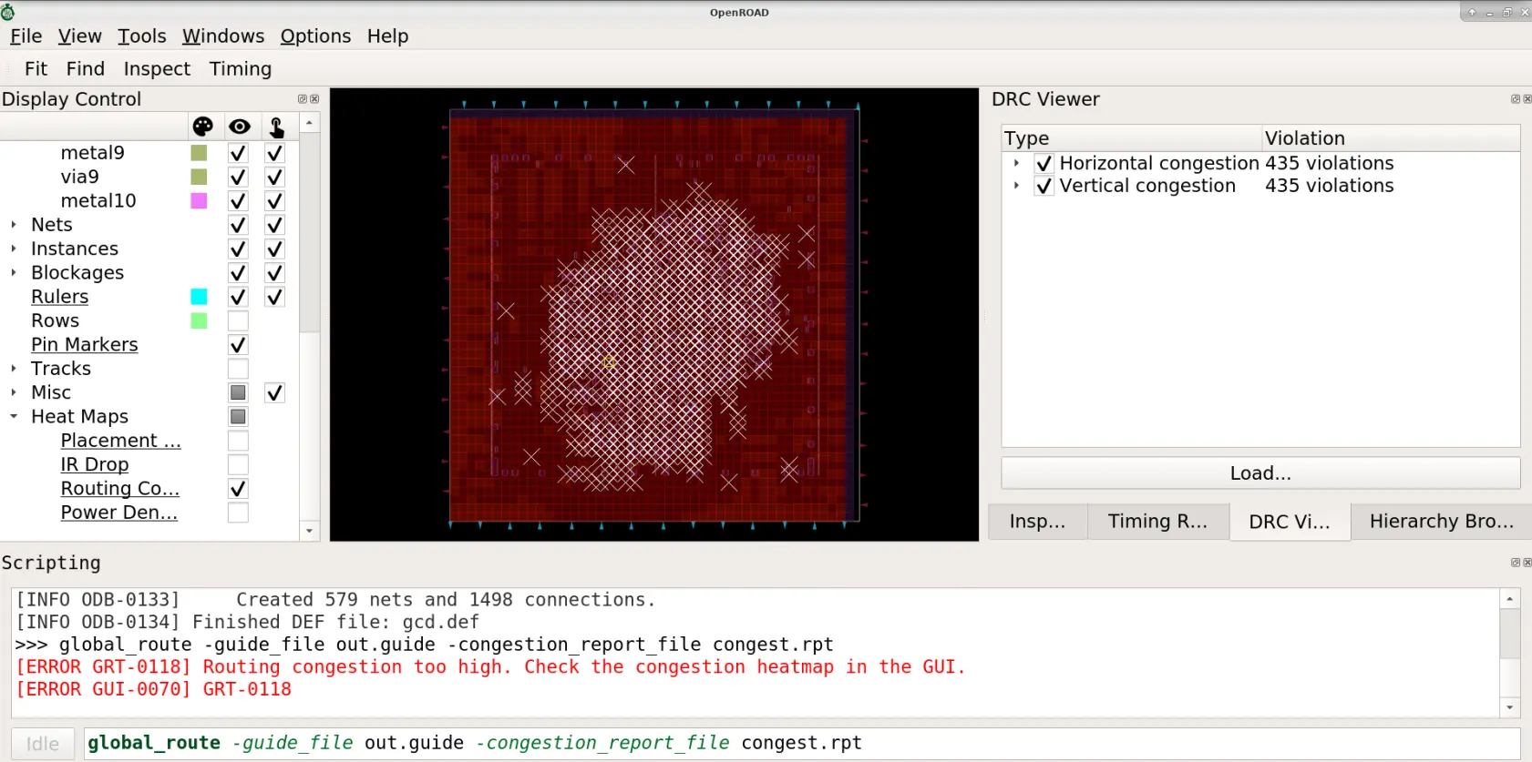
step 3: For details on the routing resources information, use the Inspector window.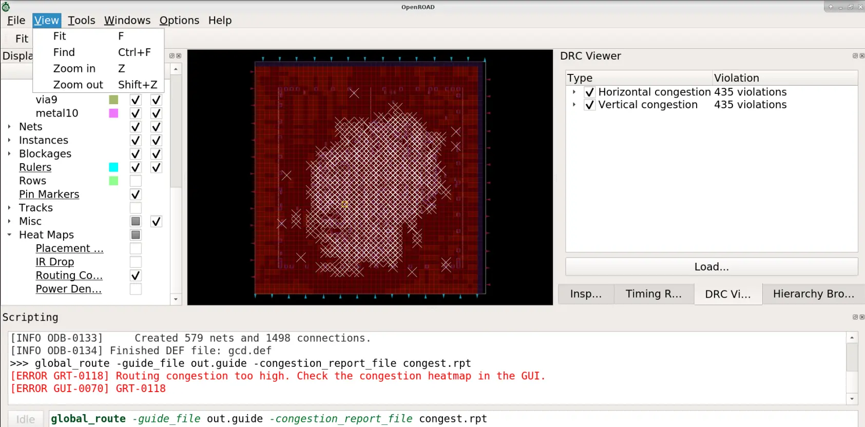

By Clicking zoom_to options, you can enlarge the view as follows: zoomto_gcell

OpenROAD Flow Scripts Tutorial

Contents

OpenROAD Flow Scripts Tutorial#

Introduction#

User Guidelines#

Getting Started#

Setting Up The Environment#

OpenROAD-flow-scripts Installation#

Running OpenROAD-flow-scripts inside the Docker#

Verifying the Docker based Installation#

Configuring The Design#

Platform Configuration#

Design Configuration#

Timing Constraints#

Design Input Verilog#

Running The Automated RTL-to-GDS Flow#

Design Goals#

Viewing OpenROAD-flow-scripts Directory Structure And Results#

Viewing Results And Logs#

Area#

Timing#

Power#

OpenROAD GUI#

Viewing Layout Results#

Visualizing Design Objects And Connectivity#

Tracing The Clock Tree#

Using Heat Maps#

Viewing Timing Report#

Using Rulers#

DRC Viewer#

Tcl Command Interface#

Customizing The GUI#

Understanding and Analyzing OpenROAD Flow Stages and Results#

Synthesis Explorations#

Area And Timing Optimization#

Floorplanning#

Floorplan Initialization Based On Core And Die Area#

Floorplan Based On Core Utilization#

IO Pin Placement#

Chip Level IO Pad Placement#

Power Planning And Analysis#

IR Drop Analysis#

Tapcell insertion#

Tie Cells#

Macro or Standard Cell Placement#

Macro Placement#

Macro Placement With Halo Spacing#

Defining Placement Density#

Timing Optimizations#

Timing Optimization Using repair_design#

Timing Optimization Using repair_timing#

Timing Optimization Based On Multiple Corners#

Fixing Setup Violations#

Fixing Hold Violations#

Clock Tree Synthesis#

Reporting Clock Skews#

Reporting CTS Metrics#

Adding Filler Cells#

Global Routing#

Detail Routing#

Antenna Checker#

Metal Fill#

Parasitics Extraction#

Troubleshooting Problems#

Debugging Problems in Global Routing#

Dump congestion information to a text file#

Visualization of overflowing GCells as markers#